SVDQuartets Lab
Up to the Phylogenetics main page
Goals
The goal of this lab exercise is to introduce you to species tree estimation with SVDQuartets.
We will be using a tutorial developed by Laura Kubatko and David Swofford for the annual Workshop in Molecular Evolution, but (in addition to PAUP*) this tutorial makes use of the software RAxML and ASTRAL, both of which you will need to install.
Answer template
Here is a text file template in which to store your answers to the ![]() thinking questions:
thinking questions:
Part 1: Analysis of a data set simulated from the “anomaly zone"

1. Which model was chosen by the AIC criterion?
answer:

2. What is the newick tree description for the concatenated analysis tree topology?
answer:

3. What is the newick tree description for the SVDQuartets tree topology?
answer:

4. What are the bootstrap percentages that are greater than 50% and thus are shown in the majority-rule consensus tree? Please indicate the splits to which these bootstrap percentages apply.
answer:

Part 2: Analysis of a real data set

5. Use PAUP*'s savetrees command to save the SVDQuartets tree using the "altnexus" format, then copy the newick tree description as your answer to this "question"
answer:

6. Use PAUP*'s qage command to save the SVDQuartets tree with estimated edge lengths to a file (specify `bootstrap=no treefile=qagetree.txt` this time but leave other settings the same), then copy the newick tree description as your answer to this "question"
answer:

7. Using the coalescent units table, which internal edge in the tree is expected to exhibit the **greatest** number of deep coalescences?
answer:

8: Which internal edge in the tree is expected to exhibit the **fewest** deep coalescences?
answer:

9. Copy the newick tree description output by ASTRAL as the answer to this "question"
answer:
Getting started
![]() Login to your account on the Storrs HPC cluster and start an interactive slurm session. If you have updated your
Login to your account on the Storrs HPC cluster and start an interactive slurm session. If you have updated your gensrun alias, you can just type:
ssh hpc
gensrun
Otherwise, type
ssh hpc
srun -p general -q general --mem=5G --pty bash
Create a directory
Use the unix mkdir command to create a directory to play in today:
cd
mkdir svdlab
cd svdlab
Load module needed
![]() We will load the following R module not because we are using R today but because this will also load gcc/11.3.0. GCC (Gnu Compiler Collection) is a C/C++ compiler (a program that turns English-like C or C++ source code into a sequence of 0s and 1s that is what the processor executes). Since we’ve used this version of GCC for other labs, it makes sense to use it for compiling the software we’re using today.
We will load the following R module not because we are using R today but because this will also load gcc/11.3.0. GCC (Gnu Compiler Collection) is a C/C++ compiler (a program that turns English-like C or C++ source code into a sequence of 0s and 1s that is what the processor executes). Since we’ve used this version of GCC for other labs, it makes sense to use it for compiling the software we’re using today.
module load r/4.3.2
Install RAxML
RAxML is one of two dominant programs for large-scale maximum likelihood phylogenetic inference. For small numbers of taxa, PAUP* performs a more thorough search for the maximum likelihood tree, but PAUP*’s search methods don’t scale well to large numbers of taxa. While we could use IQ-TREE today instead of RAxML, we’ll use RAxML because
- the tutorial uses it
- PAUP* is set up to call RAxML automatically (but not IQ-TREE), and
- this provides a good opportunity to get RAxML installed so that you have the option of using it in the future.
![]() On your laptop, open a browser and navigate to the RAxML web site.
On your laptop, open a browser and navigate to the RAxML web site.
![]() Click on the “Source Code” link in the DOWNLOAD section on the left. This will take you to the RAxML GitHub site.
Click on the “Source Code” link in the DOWNLOAD section on the left. This will take you to the RAxML GitHub site.
![]() On the right side of the GitHub page, you will see a “Releases” section. Click on the “Latest” link (this was v8.2.13 at the time of this writing):
On the right side of the GitHub page, you will see a “Releases” section. Click on the “Latest” link (this was v8.2.13 at the time of this writing):
![]() Copy the link address for Source code (tar.gz)
Copy the link address for Source code (tar.gz)
![]() Back on the cluster (in your svdlab directory), type the following **but replace
Back on the cluster (in your svdlab directory), type the following **but replace
curl -LO <RAxML tar.gz link>
I’ll assume that the file downloaded was named v8.2.13.tar.gz. The “gz” ending tells you that the file is compressed (using the gzip algorithm) and the “tar” part of the name tells you that it is a tape archive (a sequential concatenation of all files in a directory).
![]() Verbosely (
Verbosely (v) uncompress (z) and unarchive (x) the file (f) v8.2.13.tar.gz:
tar zxvf v8.2.13.tar.gz
![]() Use
Use cd to navigate into the standard-RAxML-8.2.13 directory.
cd standard-RAxML-8.2.13
ls
The ls command will reveal quite a large diversity of makefiles as well as a README.md file. Taking advice from the README.md file, let’s use the makefile named Makefile.SSE3.gcc to compile RAxML:
make -f Makefile.SSE3.gcc
If the compile takes longer than a minute, use Ctrl-C to stop it and copy the file from the /scratch/ directory, where we have placed a pre-compiled copy, to your bin directory:
cp /scratch/pol02003/pol02003/raxmlHPC-SSE3 ~/bin
![]() Test to see if RAxML is installed correctly by typing
Test to see if RAxML is installed correctly by typing
raxmlHPC-SSE3
You should see the following error message (don’t worry about the error, we’re just checking to see if it will run):
Error, you must specify a model of substitution with the "-m" option
![]() Once you verify that you have a running RAxML program, you can delete the tar.gz file and source code directory:
Once you verify that you have a running RAxML program, you can delete the tar.gz file and source code directory:
rm -rf v8.2.13.tar.gz standard-RAxML-8.2.13
![]() Finally, we will create something known as a symbolic link to the file raxmlHPC-SSE3. A symbolic link in Linux (or other Unix operating systems) is an alias or nickname for a file. The tutorial that you will follow today assumes that the RAxML executable file is named raxmlHPC and thus things will not work unless we make a symbolic link named raxmlHPC that points to the file _raxmlHPC-SSE3. Here’s how to create the symbolic link:
Finally, we will create something known as a symbolic link to the file raxmlHPC-SSE3. A symbolic link in Linux (or other Unix operating systems) is an alias or nickname for a file. The tutorial that you will follow today assumes that the RAxML executable file is named raxmlHPC and thus things will not work unless we make a symbolic link named raxmlHPC that points to the file _raxmlHPC-SSE3. Here’s how to create the symbolic link:
cd ~/bin
ln -s raxmlHPC-SSE3 raxmlHPC
This says to make a link (ln) that is symbolic (-s) to the actual file raxmlHPC-SSE3 and name the symbolic link raxmlHPC. If you type ls now you will see what the entry for a symbolic link looks like compared to the entry for an actual file:
ls -la raxml*
![]() Test to see if the symbolic link works correctly:
Test to see if the symbolic link works correctly:
cd ~/svdlab
raxmlHPC
You should (once again) see the following error message:
Error, you must specify a model of substitution with the "-m" option
Install ASTRAL
ASTRAL is a very popular program for estimating a species tree given a set of gene trees. While it is often referred to as a “coalescent” approach, its only connection to the multispecies coalescent (MSC) model is that, under the MSC, one expects the most common gene tree topology to be the species tree topology if considering only 4-taxon unrooted trees. Unlike methods that do implement the MSC model, ASTRAL never considers the original sequence data; instead, it assumes that the gene tree for each locus is known without error. While ASTRAL itself is very fast, the “prep” time required to estimate gene trees for each locus should be factored in when comparing ASTRAL’s speed to approaches such as SVDQuartets.
![]() On your laptop, navigate to the ASTRAL GitHub page
On your laptop, navigate to the ASTRAL GitHub page
![]() On the right side of the page, you should see a section named “Releases”. Click on the “Latest” release (this was v5.7.1 at the time of this writing)
On the right side of the page, you should see a section named “Releases”. Click on the “Latest” release (this was v5.7.1 at the time of this writing)
![]() Copy the link address for Source code (tar.gz)
Copy the link address for Source code (tar.gz)
Back on the cluster (in your svdlab directory), type the following **but replace
curl -LO <ASTRAL tar.gz link>
I’ll assume that the file downloaded was named v5.7.1.tar.gz.
![]() Back on the cluster, uncompress and untar the v5.7.1.tar.gz file as we did for RAxML
Back on the cluster, uncompress and untar the v5.7.1.tar.gz file as we did for RAxML
tar zxvf v5.7.1.tar.gz
![]() Use
Use cd to navigate into the ASTRAL-5.7.1 directory.
cd ASTRAL-5.7.1
ls
![]() Unzip the Astral.5.7.1.zip directly into your bin directory (note that you could have read the README.md to find installation instructions):
Unzip the Astral.5.7.1.zip directly into your bin directory (note that you could have read the README.md to find installation instructions):
unzip -d ~/bin Astral.5.7.1.zip
Unlike RAxML, which is written in the computing language C and must be compiled, ASTRAL is written in Java and does not need to be compiled before running.
![]() Test to see if ASTRAL is installed correctly by typing
Test to see if ASTRAL is installed correctly by typing
java -jar ~/bin/Astral/astral.5.7.1.jar
You should see the following error message:
bash: java: command not found
Unlike RAxML, where we ignored the error message, this error message is telling us that we do not have Java installed and therefore ASTRAL (a Java program) cannot be run.
![]() Fortunately, it is possible to “install” Java by simply loading the openjdk module:
Fortunately, it is possible to “install” Java by simply loading the openjdk module:
module load openjdk
Now the java -jar ~/bin/Astral/astral.5.7.1.jar command should work.
![]() Once you verify that you have a running ASTRAL program, you can delete the tar.gz file and source code directory:
Once you verify that you have a running ASTRAL program, you can delete the tar.gz file and source code directory:
rm -rf v5.7.1.tar.gz ASTRAL-5.7.1
Finally, we will create an alias that will issue the entire command above whenever the word astral is typed at the command line.
![]() Use nano to open the file ~/.bashrc and add the following line at the end of the file:
Use nano to open the file ~/.bashrc and add the following line at the end of the file:
alias astral='java -jar ~/bin/Astral/astral.5.7.1.jar'
![]() In order for the alias to take effect, you will need to either logout from the cluster or, alternatively, type this command, which causes the .bashrc file to be re-executed (it is normally executed when you login):
In order for the alias to take effect, you will need to either logout from the cluster or, alternatively, type this command, which causes the .bashrc file to be re-executed (it is normally executed when you login):
. ~/.bashrc
Now, if you enter astral at the command line (assuming the openjdk module is loaded), you will start ASTRAL.
Download the files for the tutorial
![]() On the cluster, in your ~/svdlab directory, use
On the cluster, in your ~/svdlab directory, use cp to copy a zip file containing the files that will be accessed during the tutorial:
cp /scratch/pol02003/pol02003/svdquartets_tutorial.zip .
![]() Unzip the files as follows:
Unzip the files as follows:
unzip svdquartets_tutorial.zip
![]() Navigate into the svdquartets_tutorial folder:
Navigate into the svdquartets_tutorial folder:
cd svdquartets_tutorial
Start the tutorial
Parts 1 and 2 of the SVDQuartets tutorial (written by David L. Swofford and Laura Kubatko) from the Woods Hole Workshop in Molecular Evolution have been recreated below (slightly modified). The bibliographic entries for literature cited in the tutorial are provided in the papers cited section of this web site.
![]() Note that (because it is a tutorial written by others) the following does not have the usual
Note that (because it is a tutorial written by others) the following does not have the usual ![]() emojis indicating when an action is required of you. However, we have sprinkled some
emojis indicating when an action is required of you. However, we have sprinkled some ![]() questions to help you keep track of what you’ve learned as you go along.
questions to help you keep track of what you’ve learned as you go along.
Preliminaries
In the instructions which follow, the $ represents the Unix prompt. For example, if the instruction says:
$ cat filename.txt
you would type cat filename.txt and hit return. Likewise, paup> represents the prompt used by the PAUP* program.
If you have not already done so, install FigTree on your local machine. FigTree is not a critical component of the tutorial however, so don’t sweat it if you run into problems.
Part 1: Analysis of a data set simulated from the “anomaly zone”
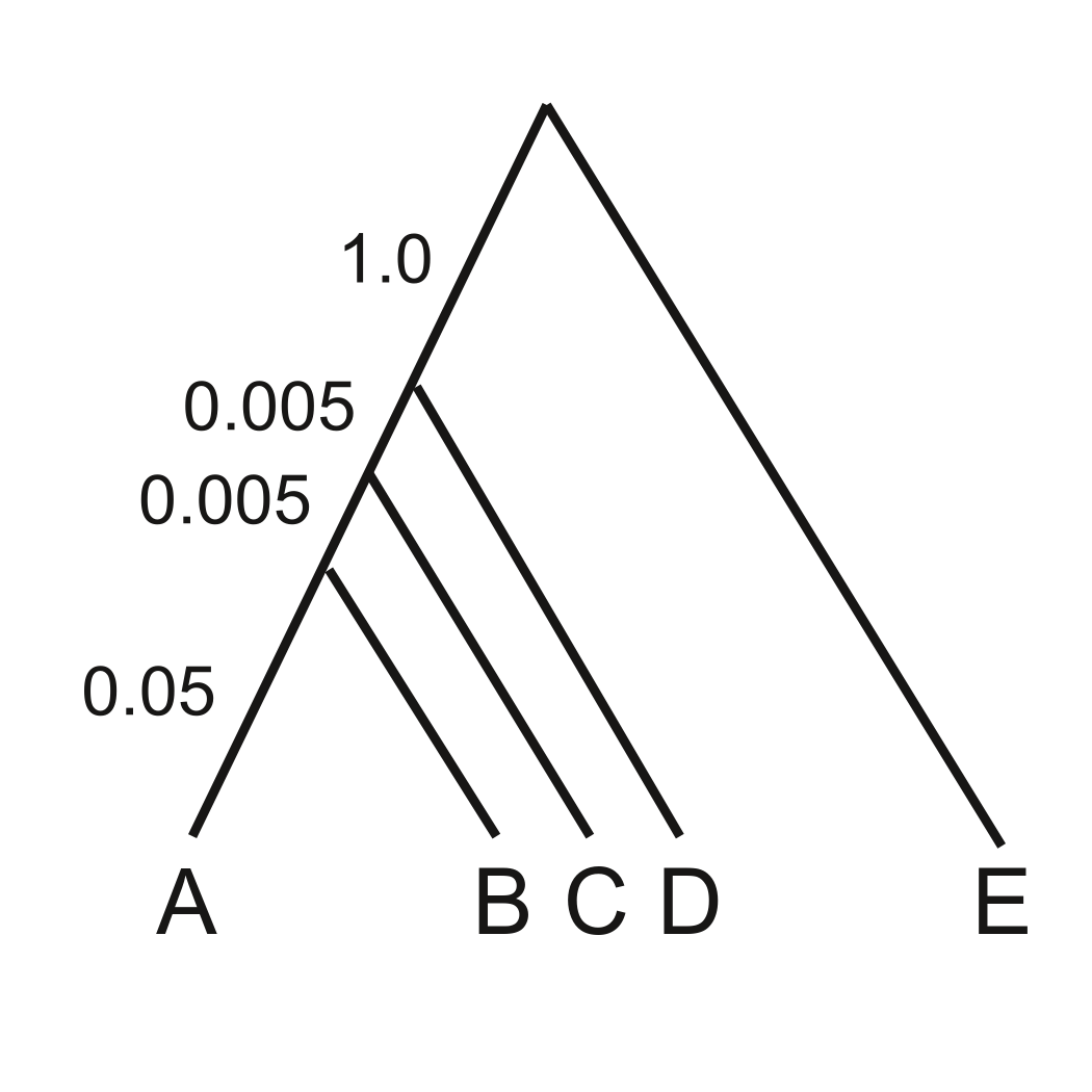
We will begin with an example used by Liu and Edwards (2009), calling attention to problems that can arise due to gene trees for individual loci conflicting with the species tree because of “incomplete lineage sorting” (ILS). When internal branches of the species tree are very short (or effective population sizes are extremely large), the most probable gene tree can be inconsistent with the species tree, which can cause “concatenation” methods for inferring the tree to fail. See Kubatko and Degnan (2007), Liu and Edwards (2009), and Roch and Steel (2015) for details.
The data file anomaly_zone.nex represents one replicate of a simulation described in Fig. 2 in Liu and Edwards (2009) (Note added by Paul and Analisa: the true tree used for the simulations is shown in the figure). This file contains data for 10,000 loci, with 500 sites per locus. We will use the PAUP* program (https://paup.phylosolutions.com/) to analyze this data set (PAUP* will subsequently be referred to as PAUP, without the asterisk). It is often convenient to run PAUP from a Nexus-file script containing the commands used to perform the analysis, but we will usually issue the commands interactively here for pedagogic reasons.
Start PAUP and load the data file.
$ paup anomaly_zone.nex -L anomaly.log
The first command argument above is the name of the data file, and the -L option opens a log file that will preserve all of the output of your run (you can use any name you like).
We’ll begin with a “concatenated” maximum-likelihood analysis to demonstrate the problem. In order to perform ML in PAUP, you first need to estimate a substitution model, which specifies the rate of substitution from each nucleotide to each other nucleotide, the equilibrium base frequencies, and the distribution of rate variation across sites. PAUP provides a tool to automatically compare models using the AIC or BIC model selection criteria. A reasonable starting tree is needed (but the details of the tree topology have little effect on the chosen model). We’ll just do a quick neighbor-joining analysis using LogDet distances (which are a good general purpose distance when you don’t know what else to use):
paup> dset distance=logdet;
paup> nj;
paup> automodel;
Using the default options, automodel will evaluate a set of 56 models and choose the one with that minimizes the AIC.
![]() Which model was chosen by the AIC criterion?
Which model was chosen by the AIC criterion?
On completion, the model parameters will be set to their maximum-likelihood estimates, and we can use this as the starting point for a maximum-likelihood search:
paup> set criterion=likelihood;
paup> hsearch;
(Note that you can abbreviate PAUP commands as long as they do not become ambiguous. For instance, instead of the above, we could have instead used set crit=like; hs;)
One way to see the tree found by the ML search is to use the describetrees command, with branch lengths drawn proportionally to the estimated number of substitutions/site:
paup> describe/plot=p;
Note the relationships among the taxa implied by the topology of this tree.
![]() What is the newick tree description for the concatenated analysis tree topology? (Note: you’ll have to use the
What is the newick tree description for the concatenated analysis tree topology? (Note: you’ll have to use the savetrees command to save the tree to a file (with a name of your choosing), specifying the “altnexus” format and that branch lengths should be saved; open the file you saved and copy the tree description out of it.)
Now we’ll do an svdquartets analysis (Chifman and Kubatko, 2014, 2015) for the same data. For any command in PAUP, you can see the available options by typing command-name ?;
Before we start our next analysis, look at the options available for the svdquartets command:
paup> help svdquartets;
For example, you can see that it is possible to evaluate quartets exhaustively (evalquartets=all) or sample quartets randomly (evalquartets=random nquartets=n). Typically, you will leave most options set at their default settings, and enter values only for those you wish to override. One exception is that the current default setting for evalquartets is random (this may change in a future version), so we will explicitly request evaluation of all possible quartets. We’ll also do a bootstrap analysis to assess confidence in the result:
paup> svdq evalq=all bootstrap;
The analysis finishes quickly and outputs the estimated tree, which is the one compatible with all 5 of the inferred quartet relationships. In fact, this is the correct tree that generated the data (see Liu and Edwards, 2009). The concatenated ML method estimated the tree incorrectly despite the large number of sites (500,000).
![]() What is the newick tree description for the SVDQuartets tree topology?
What is the newick tree description for the SVDQuartets tree topology?
![]() What are the bootstrap percentages that are greater than 50% and thus are shown in the majority-rule consensus tree? Please indicate the splits to which these bootstrap percentages apply.
What are the bootstrap percentages that are greater than 50% and thus are shown in the majority-rule consensus tree? Please indicate the splits to which these bootstrap percentages apply.
ASTRAL (Mirarab et al., 2014, 2015) is a “summary” method for estimating species trees from a set of gene trees estimated for each locus. Although it is very fast once the gene trees have been estimated, the preliminary phase of gene tree estimation (outside of ASTRAL) can take a long time. We’ll use the RAxML program (https://sco.h-its.org/exelixis/web/software/raxml/index.html) to estimate these trees (PAUP could also be used to estimate the trees, but if you have a data set with many tips, RAxML is much faster, and this example will show you how to do it.)
PAUP now provides a wrapper for RAxML that simplifies the process of obtaining the gene trees. We wrote a small Python script to generate the PAUP commands; take a quick look at it:
paup> !cat astral_prep.py
Commands typed at the command line beginning with ! are passed to a Unix shell, so this command just shows the contents of the file on your terminal. The Python program just loops through the loci and outputs commands that analyze the data for each locus.
You will remain in the shell until you hit the return key at the ! prompt, so do this now. Now run the python script from the paup> prompt to generate a Nexus command file, and hit return to go back to PAUP.
paup> !python3 astral_prep.py > run_astral.nex
The created Nexus file simply defines a “character partition” specifying the site numbers for each locus and runs a set of three commands for each of the 10,000 loci, e.g.:
include loci.locus_130/only;
raxml exec=raxmlHPC;
savetree file=az_tree.tre format=newick append;
For each locus, all of the sites except those belonging to that locus are excluded, RAxML is executed using PAUP’s current model settings, and the resulting tree is appended to a growing treefile that will ultimately contain one tree for each locus.
Now run the Nexus command file generated by the Python script (you will be warned that you are going to reset the active data file; this is fine). Running the full analysis would take several hours, so read ahead rather than waiting for the command to complete.
paup> execute run_astral.nex;
Abort the command by typing ctrl-C after a few trees have been generated. Scroll back in the output and notice how different the trees are from one locus to the next. This variation comes from two sources: (1) the true variation in gene trees coming from the multispecies coalescent process, and (2) error in estimating the gene trees using a relatively small amount of sequence information per locus.
We will pretend that the analysis actually completed, and then quit the program.
paup> quit;
As in all good cooking shows, we have pre-baked the result so that we can pull it out of the oven immediately. It is stored in the file az_10000_trees.tre, which contains one tree for each of the 10,000 trees, written in the “Newick” (nested parentheses) format. It looks like this:
    (A,(B,(D,E)),C);
    (A,((B,D),E),C);
    (A,((B,D),C),E);
    (A,(B,(D,E)),C);
    (A,((B,E),D),C);
         .
         .
         .
We’ll now run this file in ASTRAL. First, look at the options available:
$ astral --help
For now, we will simply use the default settings to estimate a species tree, using the treefile we generated above as input.
$ astral -i az_10000_trees.tre
The analysis runs quickly and outputs a few lines of output. The estimated species tree is found near the end of the output, and looks something like this:
(A,(B,(C,(E,D)1:0.025494729020277836)1:0.033915343495063886));
Like SVDQuartets, ASTRAL infers the (unrooted) species tree correctly. Note the line near the top: “All output trees will be arbitrarily rooted at A”. Both the input to and output from ASTRAL are unrooted trees; the rooting implied by the result is meaningless. In our case, the outgroup is tip E, so we would need to reroot the tree appropriately for a figure.
To view the tree, copy the output tree description the clipboard (e.g., ctrl-C), launch FigTree and paste the clipboard contents (e.g., ctrl-V). Select the terminal branch leading to tip E, and click the Reroot tool.
If you want to gain more familiarity with ASTRAL (after our practical session ends), you can run the tutorial at https://github.com/smirarab/ASTRAL/blob/master/astral-tutorial.md.
Part 2: Analysis of a real data set
The data set is for members of the family Canidae (dogs, wolves, coyotes, foxes, jackals, etc.). Lindblad-Toh et al. (2005) sequenced a collection of 16 nuclear loci. The alignments used here are from a *BEAST2 tutorial written by Huw Ogilvie. We reformatted them into the Nexus format and renamed the taxa from scientific to common names.
(Note added by Paul and Analisa: please download and unzip the *BEAST tutorial above; later parts of this tutorial refer to a file, StarBEAST2-tutorial.pdf, that you will have once you unzip the *BEAST tutorial.)
Start PAUP and load the canid sequence data file:
$ paup canids.nex -L canids.log
This file contains data for two individuals from each species (total 16 sequences), so we use a taxon-partition to assign each individual tip to a species. This definition is already in the file and you do not need to type it here. It looks like this:
taxpartition species =
    sidestriped_jackal:  sidestriped_jackal_a sidestriped_jackal_b,
    African_golden_wolf: African_golden_wolf_a African_golden_wolf_b,
    coyote:              coyote_a coyote_b,
    gray_wolf:           gray_wolf_a gray_wolf_b,
    blackbacked_jackal:  blackbacked_jackal_a blackbacked_jackal_b,
    Ethiopian_wolf:      Ethiopian_wolf_a Ethiopian_wolf_b,
    Dhole:               Dhole_a Dhole_b,
    African_wild_dog:    African_wild_dog_a African_wild_dog_b
    ;
Analysis 1: Using SVDQuartets and qAge
Perform an SVDQuartets analysis, referencing this taxon partition:
paup> svdq nthreads=1 evalq=all taxpartition=species;
![]() Use PAUP*’s savetrees command to save the SVDQuartets tree using the “altnexus” format, then copy the newick tree description as your answer to this “question”
Use PAUP*’s savetrees command to save the SVDQuartets tree using the “altnexus” format, then copy the newick tree description as your answer to this “question”
Notice that the (North American) gray wolf (Canis lupus) joins with the African golden wolf (Canis anthus) rather than the (North American) coyote (Canis latrans), unlike the result of the *BEAST tutorial (see StarBEAST2-tutorial.pdf). However, this result is not well supported, as we can see by doing a multilocus nonparametric bootstrap, which resamples (with replacement) both loci and sites within loci:
paup> svdq nthreads=1 evalq=all taxpartition=species bootstrap=multilocus loci=combined;
(The “combined” above is the name of the character partition defining genes in the input file.) Examining the output bootstrap consensus tree, we see that the bootstrap support for the (gray wolf, African golden wolf) grouping is weak, and many bootstrap runs will actually find the (gray wolf, coyote) grouping that is probably correct. Interestingly, the DensiTree plot in the *BEAST tutorial also demonstrates that support for this grouping is very weak.
PAUP also includes a method for estimating branch lengths within a fixed species tree. The method is run with the “qAge” command, and you can find help with this command as above:
paup> help qAge;
To estimate the branch lengths under the JC69 model, we can use the commands below. The first command converts the tree estimated by SVDQuartets to a rooted tree, and the second calls qAge to estimate the branch lengths on the rooted tree. Bootstrapping is used to obtain 95% confidence intervals. We’ll take a look at the output as a group.
paup> roottrees rootmethod=outgroup;
paup> qage taxpartition=species outunits=both bootstrap=multilocus loci=combined;
![]() Use PAUP*’s qage command to save the SVDQuartets tree with estimated edge lengths to a file (specify
Use PAUP*’s qage command to save the SVDQuartets tree with estimated edge lengths to a file (specify bootstrap=no treefile=qagetree.txt this time but leave other settings the same), then copy the newick tree description as your answer to this “question”
![]() Note that PAUP* provided estimated branch lengths in two different units: substitutions/site and coalescent units. A coalescent unit is the expected time for two randomly selected genes from a population to coalesce given the effective population size. Using the coalescent units table, which internal edge in the tree is expected to exhibit the greatest number of deep coalescences? (Please don’t just give the node number: specify all taxa on one side of this edge)
Note that PAUP* provided estimated branch lengths in two different units: substitutions/site and coalescent units. A coalescent unit is the expected time for two randomly selected genes from a population to coalesce given the effective population size. Using the coalescent units table, which internal edge in the tree is expected to exhibit the greatest number of deep coalescences? (Please don’t just give the node number: specify all taxa on one side of this edge)
![]() Which internal edge in the tree is expected to exhibit the fewest deep coalescences? Again, specify the taxa on one side of the split to identify the edge.
Which internal edge in the tree is expected to exhibit the fewest deep coalescences? Again, specify the taxa on one side of the split to identify the edge.
qAge also includes an option to carry out estimation under more complex substitution models. This option is invoked by changing patProb=exactJC to patProb=expBL. Prior to doing this, however, you must define a model using the lset command and provide the name of that model to the qAge command. Below is sample code.
In the first line, we specify a GTR model, with parameters in the model to be estimated.
paup> lset nst=6 rmatrix=estimate baseFreq=empirical;
The second line asks PAUP* to estimate those parameters using our data and the current tree in memory.
paup> lscores;
In the third line, we set the model with the estimated values of the parameters, and we name it “MyGTR”.
paup> lset nst=6 rmatrix=(0.749 2.410 0.365 1.066 4.465 1.000) baseFreq=(0.2476 0.2679 0.2558 0.2286) modelName=MyGTR;
The final line uses qAge to carry out estimation under that model.
paup> qage patProb=expBL taxpartition=species loci=combined bootstrap=multilocus treefile=test.tre modelName=MyGTR poolJC=no nreps=100;
Note that this analysis is more computationally intensive than the previous one that assumes the JC69 model. If you plan to try this analysis now, you may want to reduce the number of bootstrap replicates (currently set as nreps=100).
Analysis 2: Using ASTRAL
We will again run ASTRAL so that you can see how to apply ASTRAL to an empirical data set. As before the first step is to estimate gene trees for each of the 16 loci. We can do this with the following two commands:
paup> !python3 astral_prep_canids.py > run_astral_canids.nex
paup> exec run_astral_canids.nex;
(In an interactive session you will need to hit return at the ! prompt to return to the PAUP prompt). You can ignore warnings from PAUP* about the ingroup not being monophyletic; the trees are considered to be unrooted when input to ASTRAL.
After issuing these two commands, you will have a file called canids_genetrees.tre in your directory. This file contains a gene tree for each of the 16 genes, and will be used as the input to ASTRAL. There is one more file needed to run PAUP for this data set. We need to create a file that maps individual lineages to species, similar to the “taxpartition” we created in PAUP. This file is called astral_canid_mapfile. To run ASTRAL, you can now quit PAUP, and issue the following command:
$ astral -i canids_genetrees.tre -a astral_canid_mapfile
Again, you can locate the tree in the output written to the screen.
![]() Copy the newick tree description output by ASTRAL as the answer to this “question”
Copy the newick tree description output by ASTRAL as the answer to this “question”
Copying and pasting the estimated tree into FigTree and rooting along the branch that separates the sidestriped jackal and the blackbacked jackal from the rest of the species, we see that this tree agrees with that estimated with SVDQuartets using the bootstrap and with *BEAST2.
What to turn in
Send the file with your answers to the thinking questions to Analisa on Slack to get credit.