RevBayes Divergence Dating Lab
Up to the Phylogenetics main page
Goals
The goal of this lab exercise is to introduce you to Bayesian divergence time estimation. There are other programs that are popular for divergence time analyses (notably BEAST2), but we will use RevBayes because you already have some experience with this program.
Part 1: Simulate a tree and DNA sequence data with known properties (e.g. speciation rate, nucleotide frequencies, strict molecular clock rate, etc.)
Part 2: Analyze the simulated data under a strict clock model while fixing the topology to see how well we can estimate parameters such as clock rate and speciation rate whose true values we know because we simulated the data
Part 3: Analyze the simulated data under a relaxed clock model while fixing the topology to see whether we can infer that the data were actually simulated under a strict clock
Part 4: Analyze under a relaxed clock model, this time allowing topology to vary, and estimate relative divergence times
Part 5: Compare credible intervals from part 4 to those under the prior to see whether the there is information in the data about divergence times.
We will use RevBayes to both simulate tree and data as well as for analysis of the simulated data.
Answer template
Here is a text file template in which to store your answers to the ![]() thinking questions:
thinking questions:
1. What is the true tree length? What is the estimated length of the neighbor-joining tree?
answer:

2. What are the true base frequencies? What are the estimated base frequencies?
answer:

3. What are the true exchangeabilities? What are the estimated exchangeabilities?
answer:

4. What is the 95% HPD (highest posterior density) credible interval for clock_rate (use the Estimates tab in Tracer to find this information)? Does this include the true value?
answer:

5. What is the 95% HPD (highest posterior density) credible interval for birth_rate? Does this include the true value?
answer:

6. Which parameter (clock_rate or birth_rate) is hardest to estimate precisely (i.e. has the broadest HPD credible interval)?
answer:

7. For the parameter you identified in the previous question, would it help to simulate 20000 sites rather than 10000?
answer:

8. What would help in reducing the HPD interval for birth_rate?
answer:

9. Using the 'Marginal Density" and "Estimates" tabs in Tracer, select all 6 exchangeabilities. What do these values represent, and what about these densities makes sense given what you know about the true model used to simulate the data?
answer:

10. Using the Marginal Density tab in Tracer, select all 4 state_freqs. What about these densities make sense given what you know about the true model used to simulate the data?
answer:

11. What is the true rate for any given edge in the tree?
answer:

12. Looking across the 38 branch rate parameters, do any of them get very far from 1.0 (e.g. less than 0.98 or greater than 1.2)?
answer:

13. What are the mean values of ucln_mu and ucln_sigma, our two hyperparameters that govern the assumed lognormal prior applied to each branch rate?
answer:

14. What do these values translate to on the linear scale (use the formulas in the figure to do the calculation)?
answer:

15. Do the values on the linear scale make sense in light of the fact that you know that the data were simulated under a strict clock with rate 1.0?
answer:

16. We've added moves, but no parameters or priors for the node times. Why not?
answer:

17. Does the MAP tree have the same topology as the true tree
answer:

18. Are we more confident about recent nodes or ancient nodes in the tree?
answer:

19. What would you conclude if these credible intervals were exactly the same size if we had performed the MCMC analysis on the prior only, with no data?
answer:

20. Does the data contain information about substitution rates?
answer:
Getting started
![]() Login to your account on the Storrs HPC cluster and start an interactive slurm session. If you have updated your
Login to your account on the Storrs HPC cluster and start an interactive slurm session. If you have updated your gensrun alias, you can just type:
ssh hpc
gensrun
Otherwise, type
ssh hpc
srun -p general -q general --mem=5G --pty bash
Important The --mem=5G part is important for this lab, as RevBayes sometimes uses more than the default amount of memory.
Create a directory
Use the unix mkdir command to create a directory to play in today:
cd
mkdir rbdiv
cd rbdiv
Load module needed
![]() The RevBayes executable file needs some runtime libraries that can be loaded using the module system. Loading the R module loads the runtime library needed by rb132:
The RevBayes executable file needs some runtime libraries that can be loaded using the module system. Loading the R module loads the runtime library needed by rb132:
module load r/4.3.2
![]() You should now be able to type rb132 to start the program:
You should now be able to type rb132 to start the program:
RevBayes version (1.3.2)
Build from tags/v1.3.2 (rapture-4486-g3d84ac) on Sat Feb 28 11:57:57 EST 2026

Visit the website www.RevBayes.com for more information about RevBayes.

RevBayes is free software released under the GPL license, version 3. Type 'license()' for details.

To quit RevBayes type 'quit()' or 'q()'.
Use RevBayes to simulate data under a strict molecular clock
Divergence time analyses are the trickiest type of analysis we will do in this course. That’s because the sequences do not contain information about substitution rates or divergence times per se; they contain information about the number of substitutions that have occurred, and the number of substitutions is the product of rate and time. Thus, maximum likelihood methods cannot separate rates from times; doing so requires a Bayesian approach and careful use of priors, which constrain the range of rate and time scenarios considered plausible.
We will thus start slowly, simulating data so that we know the truth. This will help guide your expectations when conducting divergence time analyses on real data.
As you already know from previous labs, RevBayes uses an R-like language called the Rev Language to specify the model and the analysis. Rev is not R, but it is so similar to R that you will often forget that you are not using R and will try things that work in R but do not work in Rev - just a heads-up!
![]() Create the file sim.Rev to create instructions for simulating a tree and DNA sequence data on that tree:
Create the file sim.Rev to create instructions for simulating a tree and DNA sequence data on that tree:
# Set the random number seed, number of sites, number of taxa, and specify taxon names
seed(12345)
printSeed()

n_sites <- 10000

n_taxa <- 20
taxon_names[1]  <- taxon("A")
taxon_names[2]  <- taxon("B")
taxon_names[3]  <- taxon("C")
taxon_names[4]  <- taxon("D")
taxon_names[5]  <- taxon("E")
taxon_names[6]  <- taxon("F")
taxon_names[7]  <- taxon("G")
taxon_names[8]  <- taxon("H")
taxon_names[9]  <- taxon("I")
taxon_names[10] <- taxon("J")
taxon_names[11] <- taxon("K")
taxon_names[12] <- taxon("L")
taxon_names[13] <- taxon("M")
taxon_names[14] <- taxon("N")
taxon_names[15] <- taxon("O")
taxon_names[16] <- taxon("P")
taxon_names[17] <- taxon("Q")
taxon_names[18] <- taxon("R")
taxon_names[19] <- taxon("S")
taxon_names[20] <- taxon("T")

# Simulate a Yule (pure-birth) tree

timetree ~ dnBirthDeath(lambda = 2.6, mu = 0.0, rho = 1.0, rootAge = 1.0, samplingStrategy = "uniform", condition = "nTaxa", taxa = taxon_names)
timetree.redraw()
print("true root age: ", timetree.rootAge())
print("true tree length: ", timetree.treeLength())

# Set up the GTR model

state_freqs <- Simplex([0.1, 0.2, 0.3, 0.4])

exchangeabilities <- Simplex([1,5,1,1,5,1])
Q := fnGTR(exchangeabilities, state_freqs)

# Simulate DNA sequence data on timetree using the GTR Q matrix

phySeq ~ dnPhyloCTMC(tree=timetree, Q=Q, branchRates=1.0, nSites=n_sites, type="DNA")
phySeq.redraw()

# Save the simulated tree
write(timetree, filename="simulated.tre")

# Save the simulated data
writeNexus("simulated.nex", phySeq)

quit()
Important: Do not change the random number seed specified above. We will thus all simulate exactly the same true tree and sequence data. This will be important later on in the lab as you will see.
![]() Run RevBayes to simulate data:
Run RevBayes to simulate data:
rb132 sim.Rev
Note that there are two redraw() calls here, one for timetree and one for phySeq. These calls each result in simulation. The timetree.redraw() simulates a tree topology and branch lengths using the Yule model (because death rate mu is set to 0.0). The phySeq.redraw() call simulates sequence data on the supplied tree and with the supplied substitution model.
RevBayes should have reported the true root age and the true treelength. These reports come from the two print calls. The root age will be 1 because we specified that in the call to dnBirthDeath.
![]() Before going further, write down the true tree length so that we can see how well this can be estimated.
Before going further, write down the true tree length so that we can see how well this can be estimated.
You should now find two new files in your rbdiv directory: simulated.tre and simulated.nex.
Let’s use PAUP* to see how well we can estimate things like the base frequencies, exchangeabilities, and tree length:
![]() Open simulated.nex in nano and add the following paup block to the end of the file to estimate parameters on a neighbor-joining tree:
Open simulated.nex in nano and add the following paup block to the end of the file to estimate parameters on a neighbor-joining tree:
begin paup;
    log start file=pauplog.txt replace;
    set crit=like nowarntsave;
    lset nst=6 basefreq=estimate rmatrix=estimate rates=equal pinvar=0;
    nj;
    lscores 1;
    describe 1 / noplot brlens=sumonly;
    log stop;
    quit;
end;
![]() Execute the file simulated.nex in PAUP* and answer the next few questions based on PAUP*’s output, which will be saved in the file pauplog.txt.
Execute the file simulated.nex in PAUP* and answer the next few questions based on PAUP*’s output, which will be saved in the file pauplog.txt.
What is the true tree length? What is the estimated length of the neighbor-joining tree?
Use RevBayes to estimate the birth rate and clock rate
In our first RevBayes analysis, we will see how well we can estimate what we already know to be true about the evolution of both the tree and the sequences. You will cheat a little bit and fix some things to their known true values, such as the tree topology and edge lengths. The idea is to take small steps so that we know what we are doing all along.
Get RevBayes running
Because this analysis takes a little while to run, let’s get it started first and, while it is running, read the following sections that explain the commands that are in the file:
![]() Create a new file named strict.Rev and add the following to it:
Create a new file named strict.Rev and add the following to it:
# Set random number seed (you can choose your own this time)
seed(13579)
printSeed()

# Load data and tree

D <- readDiscreteCharacterData(file="simulated.nex")
n_sites <- D.nchar()

T <- readTrees("simulated.tre")[1]
n_taxa  <- T.ntips()
taxa  <- T.taxa()

# Initialize move (nmoves) and monitor (nmonitors) counters

nmoves = 1
nmonitors = 1

# Birth-death tree model

death_rate <- 0.0
birth_rate ~ dnExponential(0.01)
birth_rate.setValue(1.0)
diversification := birth_rate - death_rate
moves[nmoves++] = mvSlide(birth_rate, delta=1.0, tune=true, tuneTarget=0.4, weight=1.0)
sampling_fraction <- 1.0
root_time <- T.rootAge()
timetree ~ dnBirthDeath(lambda = birth_rate,
    mu = death_rate,
    rho = sampling_fraction,
    rootAge = root_time,
    samplingStrategy = "uniform",
    condition = "nTaxa",
    taxa = taxa)
timetree.setValue(T)

# Strict clock

clock_rate ~ dnExponential(0.01)
clock_rate.setValue(1.0)
moves[nmoves++] = mvSlide(clock_rate, delta=1.0, tune=true, tuneTarget=0.4, weight=1.0)

# GTR model

state_freqs ~ dnDirichlet(v(1,1,1,1))
exchangeabilities ~ dnDirichlet(v(1,1,1,1,1,1))
Q := fnGTR(exchangeabilities, state_freqs)
moves[nmoves++] = mvDirichletSimplex(exchangeabilities, alpha=10.0, tune=true, weight=1.0)
moves[nmoves++] = mvDirichletSimplex(state_freqs, alpha=10.0, tune=true, weight=1.0)

# PhyloCTMC

phySeq ~ dnPhyloCTMC(tree=timetree, Q=Q, branchRates=clock_rate, nSites=n_sites, type="DNA")
phySeq.clamp(D)
mymodel = model(exchangeabilities)

mymodel.graph("strict.dot", TRUE, "white")

# Monitors

monitors[nmonitors++] = mnModel(filename  = "output/strict.log",  printgen = 10, separator = TAB)
monitors[nmonitors++] = mnFile(filename  = "output/strict.trees", printgen = 10, timetree)
monitors[nmonitors++] = mnScreen(printgen=100)

# MCMC

mymcmc = mcmc(mymodel, monitors, moves, nruns=1)
mymcmc.burnin(generations=1000, tuningInterval=100)
mymcmc.run(generations=10000)
mymcmc.operatorSummary()

quit()
![]() Copy the contents above into a text editor on your laptop so that you can look at it while your console window is tied up with the RevBayes run.
Copy the contents above into a text editor on your laptop so that you can look at it while your console window is tied up with the RevBayes run.
![]() To run RevBayes, enter the following at the command prompt with the name of your revscript file last:
To run RevBayes, enter the following at the command prompt with the name of your revscript file last:
rb132 strict.Rev
Understanding the RevBayes code
While RevBayes is running, read through the following sections so that you understand what it is doing.
Setting up the tree submodel
Take a look at the “Load data and tree” and “Birth-death tree model” sections of the strict.Rev file. Note that we are assigning only the first tree in simulated.tre to the variable T (there is only 1 tree in that file, but RevBayes stores the trees it reads in a vector, so you have to add the [1] to select the first anyway).
The functions beginning with dn (e.g. dnExponential and dnBirthDeath) are probability distributions. Thus, birth_rate is a parameter that is assigned an Exponential prior distribution having rate 0.01, and timetree is a compound parameter representing the tree and its branching times that is assigned a Birth Death Process (BDP) prior distribution. The BDP is a submodel, like the +I or +G rate heterogeneity submodels: it has its own parameters (lambda, mu, rho, and rootAge) all of which are fixed except for birth_rate.
The setValue function used on the last line sets the starting value of a parameter that is allowed to vary. In this case, we are using setValue to start off our MCMC analysis with the true tree and true edge lengths.
Each parameter in the model requires a mechanism to propose changes to its value during an MCMC run. These are called moves. A vector of moves has been created for you, so you need only add to it. The variable nmoves keeps track of how many moves we’ve defined. Each time a move is added to the moves vector, we increment the variable nmoves so that new moves will not overwrite previously defined moves. This increment is performed by the ++ in nmoves++. Thus, if nmoves currently has the value 2, moves[nmoves++] = ... sets the value of moves[2] to ... (not literally, of course; the ellipses stand in for whatever move you are creating) and immediately increments nmoves to 3 so it will refer to the next empty slot in the moves vector whenever we add another move.
Monitors in RevBayes handle output. We are just initializing the monitor counters now; we will add monitors toward the end of our RevBayes script.
The model can be summarized by a DAG (Directed Acyclic Graph). The nodes of this graph are of several types and represent model inputs and outputs:
-
Stochastic nodes are exemplified by
birth_rateandtimetree; they can be identified by the tilde (~) symbol used to assign a prior distribution. These quantities are parameters that will be updated during MCMC. -
Constant nodes are exemplified by
death_rate,sampling_fraction, androot_time; they can be identified by the assignment operator<-that fixes their value to a constant. They are not changed during the MCMC analysis. -
Deterministic nodes are exemplified by
diversification; they can be identified by the assignment operator:=. These nodes represent functions of other nodes used to output quantities in a more understandable way. For example, diversification (birth rate minus death rate) will show up as a column in the output even though it is not a parameter of the model itself. (The diversification node was only added here to illustrate deterministic nodes; it’s value will always equal birth_rate because death_rate is a constant 0.0).
Setting up the strict clock submodel
Now take a look at the “Strict clock” section of your strict.Rev file:
This adds a parameter clock_rate with a vague Exponential prior (rate 0.01) and starting value 1.0. The move we’re using to propose new values for this parameter as well as the birth_rate parameter is a sliding window move, which you are familiar with from your MCMC homework. The value delta is the width of the window centered over the current value, and we’ve told RevBayes to tune this proposal during the burnin period so that it achieves (if possible) an acceptance rate of 40%. The weight determines the probability that this move will be tried. At the start of the MCMC analysis, RevBayes sums the weights of all moves you’ve defined and uses the weight divided by the sum of all weights as the probability of selecting that particular move next.
Setting up the substitution submodel
The “GTR model” section of your strict.Rev file sets up a GTR substitution model.
The Q matrix for the GTR model involves state frequencies and exchangeabilities. I’ve made both state_freqs and exchangeabilities stochastic nodes in our DAG and assigned both of them flat Dirichlet prior distributions (the v(1,1,...,1) part is the vector of parameters for the Dirichlet prior distribution (all 1s produces a flat prior distribution in which every possible combination of state frequencies (or exchangeabilities) is equally probable).
I’ve assigned mvDirichletSimplex moves to both of these parameters. A simplex is a set of coordinates that are constrained to sum to 1, and this proposal mechanism modifies all of the state frequencies (or exchangeabilities) simultaneously while honoring this constraint. A list of all available moves can be found in the Documentation section of the RevBayes web site if you want to know more.
Finalize the PhyloCTMC
The “PhyloCTMC” section collects the various submodels (timetree, Q, and clock_rate) into one big Phylogenetic Continuous Time Markov Chain (dnPhyloCTMC) distribution object and attaches (clamps) the data matrix D to it.
The last line in this section is a little obscure. RevBayes needs to have an entry point (a root node, if you will) into the DAG, and any stochastic node will suffice. Here I’ve supplied exchangeabilities when constructing mymodel, but I could have instead provided state_freqs, birth_rate, clock_rate, or any other variable representing a node in the DAG.
The mymodel.graph line creates a file named strict.dot that contains code (in the dot language) for creating a plot of your DAG. The second argument (TRUE) tells the graph command to be verbose, and the last argument (“white”) specifies the background color for the plot.
Setting up monitors
The “Monitors” section creates 3 monitors to keep track of sampled parameter values, sampled trees, and screen output:
The first monitor will save model parameter values to a file named strict.log in the output directory (which will be created if necessary). The second monitor will save trees to a file named strict.trees in the output directory. Note that we have to give it timetree as an argument. This is kind of silly because we’ve fixed the tree topology and edge lengths, so all the lines in the strict.trees will be identical, but let’s add it anyway just as a sanity check to verify that the tree topology and edge lengths don’t change during the MCMC run. Finally, the third monitor produces output to the console so that you can monitor progress.
Note that we are sampling only every 10th iteration for the first 2 monitors and every 100th iteration for the screen monitor.
Set up MCMC
Finally, the “MCMC” section creates an mcmc object that combines the model, monitors, and moves and says to do just 1 MCMC analysis. We will devote the first 1000 iterations to burnin, stopping to tune the moves every 100 iterations (RevBayes collects data for 100 iterations to compute the acceptance probabilities for each move, then uses that to decide whether to make the move bolder or more conservative.) Then we run for real for 10000 iterations and ask RevBayes to output an operator summary, which will tell us how often each of our moves was attempted and succeeded.
Reviewing the strict clock results
Hopefully your RevBayes run has now finished. If not, wait here until it is done.
![]() Before doing anything else, use nano to create a file named operator-summary-strict.txt and copy into it the operator summary table at the end of the RevBayes output so that you can refer to it later.
Before doing anything else, use nano to create a file named operator-summary-strict.txt and copy into it the operator summary table at the end of the RevBayes output so that you can refer to it later.
nano operator-summary-strict.txt
![]() Copy the contents of the file strict.dot and paste them into one of the online Graphviz viewers such as GraphvizFiddle, GraphvizOnline, or WebGraphviz.
Copy the contents of the file strict.dot and paste them into one of the online Graphviz viewers such as GraphvizFiddle, GraphvizOnline, or WebGraphviz.
The resulting plot shows your entire model as a graph, with constant nodes in square boxes, stochastic nodes in solid-line ovals, and deterministic nodes in dotted-line ovals.
![]() Download the file strict.log stored in the output directory to your laptop and open it in Tracer.
Download the file strict.log stored in the output directory to your laptop and open it in Tracer.
You may have noticed that our effective sample sizes for the exchangeabilities and state_freqs parameters are pretty low (Tracer colors them **red>/span>** to signify that they are dangerously low). You no doubt also noticed that these are being estimated quite precisely and accurately. What gives? The fact that there is so much information in the data about these parameters is the problem here. The densities for these parameters are very sharp (low variance), and proposals that move the values for these parameters away from the optimum by very much fail.
Looking at the operator summary table generated after the MCMC analysis finished (which you stored in the operator-summary.txt file), you will notice that RevBayes maxed out its tuning parameter (alpha) for both exchangeabilities and state_freqs at 100. Making this tuning parameter larger results in smaller proposed changes, so if we could set the tuning parameter alpha to, say, 1000 or even 10000, we could achieve better acceptance rates and higher ESSs.
Relaxed clocks
It is safe to assume that a strict molecular clock almost never applies to real data (although it does apply to our simulated data). So, it would be good to allow some flexibility in rates. One common approach is to assume that the rates for each edge are drawn from a lognormal distribution. This is often called an UnCorrelated Lognormal (UCLN) relaxed clock model because the rate for each edge is independent of the rate for all other edges (that’s the uncorrelated part) and all rates are lognormally distributed. This is to distinguish this approach from correlated relaxed clock models, which assume that rates are to some extent inherited from ancestors, and thus there is autocorrelation across the tree.
![]() Copy your strict.Rev script to a file named relaxed.Rev:
Copy your strict.Rev script to a file named relaxed.Rev:
cp strict.Rev relaxed.Rev
![]() Edit relaxed.Rev in nano, replacing the section entitled “Strict clock” with this relaxed clock version:
Edit relaxed.Rev in nano, replacing the section entitled “Strict clock” with this relaxed clock version:
# Uncorrelated Lognormal relaxed clock

# Add hyperparameters mu and sigma
ucln_mu ~ dnNormal(0.0, 100)
ucln_sigma ~ dnExponential(.01)
moves[nmoves++] = mvSlide(ucln_mu,    delta=0.5, tune=true, tuneTarget=0.4, weight=1.0)
moves[nmoves++] = mvSlide(ucln_sigma, delta=0.5, tune=true, tuneTarget=0.4, weight=1.0)

# Create a vector of stochastic nodes representing branch rate parameters
n_branches <- 2*n_taxa - 2
for(i in 1:n_branches) {
    branch_rates[i] ~ dnLognormal(ucln_mu, ucln_sigma)
    branch_rates[i].setValue(1.0)
    moves[nmoves++] = mvSlide(branch_rates[i], delta=0.5, tune=true, weight=1.0)
}
![]() You’ll also need to substitute
You’ll also need to substitute branch_rates for clock_rate in your dnPhyloCTMC call…
phySeq ~ dnPhyloCTMC(tree=timetree, Q=Q, branchRates=branch_rates, nSites=n_sites, type="DNA")
The model has suddenly gotten a lot more complicated, hasn’t it? We now have a rate parameter for every edge in the tree, so we’ve added \((2)(20) - 2 = 38\) more parameters to the model. Each of these edge rate parameters has a lognormal prior, and the 2 parameters of that distribution represent hyperparameters in what is now a hierarchical model, so we’ve increased the model from 10 parameters (1 clock_rate, 1 birth_rate, 3 state_freqs, 5 exchangeabilities) to 50 parameters (the original 10 plus 38 edge rates and 2 hyperparameters ucln_mu and ucln_sigma).
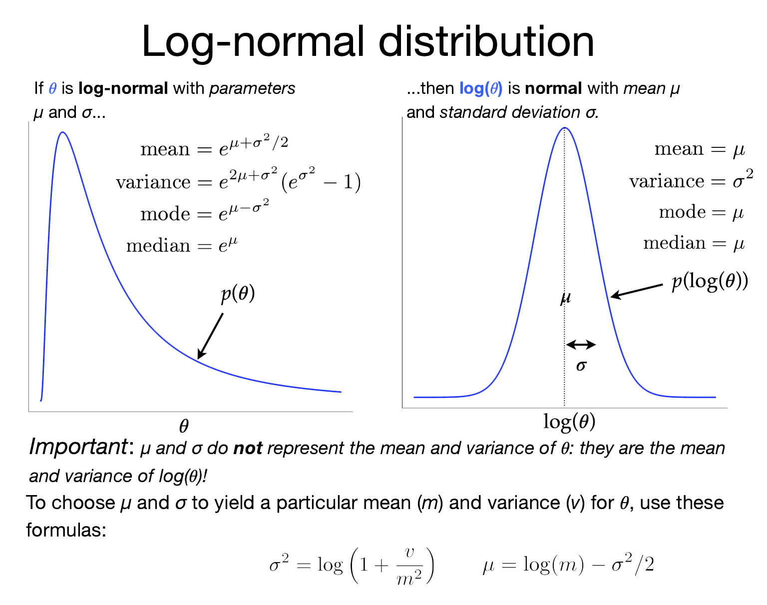
The image on the right shows the relationship between the lognormal distribution (left) and the normal distribution (right). The lognormal distribution is tricky in that its two parameters (\(\mu\) and \(\sigma\)) are not the mean and standard deviation of the lognormally-distributed variable, as you might be led to assume if you are used to the \(\mu\) and \(\sigma\) associated with normal distributions. In a Lognormal distribution, \(\mu\) and \(\sigma\) are, instead, the mean and standard deviation of the log of the lognormally-distributed variable!
Note this line:
branch_rates[i].setValue(1.0)
This sets the starting value of all branch rate parameters to 1.
This seems to be kind of important. If you let RevBayes choose starting values for branch rates, it will start by drawing values for hyperparameters ucln_mu and ucln_sigma (which, due to the high variances we’ve given to their hyperpriors, can result in some pretty crazy values) and then will draw values from Lognormal(ucln_mu, ucln_sigma) to serve as starting values for the branch rates. This procedure could start us very far away from a reasonable constellation of parameter values and the MCMC analysis may never find its way to a reasonable configuration, at least with the length of run we are able to manage in a lab period.
Unless you are particularly interested in how well your MCMC converges from diverse starting points, it is a good idea to start an MCMC analysis with all parameters set to reasonable values, for example maximum likelihood estimates (MLEs). This does not violate Bayesian principles in any way, and it saves on the amount of burnin that needs to be done. This is especially true for complex models where the amount of information for estimating parameters is low. Here I’m cheating a bit and setting the branch rates to what I know is the true value (1.0), but if we used our estimated clock_rate from the previous analysis things would work out just as well.
![]() You should also edit the monitors section so that the output file names reflect the fact that we’re using a relaxed clock now:
You should also edit the monitors section so that the output file names reflect the fact that we’re using a relaxed clock now:
# Monitors

monitors[nmonitors++] = mnModel(filename  = "output/relaxed.log",  printgen = 10, separator = TAB)
monitors[nmonitors++] = mnFile(filename  = "output/relaxed.trees", printgen = 10, timetree)
monitors[nmonitors++] = mnScreen(printgen=100)
![]() And don’t forget to change the name of the dot file:
And don’t forget to change the name of the dot file:
mymodel.graph("relaxed.dot", TRUE, "white")
![]() Now run the new model:
Now run the new model:
rb132 relaxed.Rev
Review results of the relaxed clock analysis
If you create a plot of your relaxed.dot file using one of the online Graphviz viewers, the increase in model complexity will be very apparent!
![]() Open the relaxed.log file in Tracer and answer the following questions:
Open the relaxed.log file in Tracer and answer the following questions:
Divergence times
So far we’ve not estimated any divergence times! We’ve assumed the true tree topology and true divergence times for all of our analyses. In reality, our main interest probably lies in estimating divergence times. We don’t really care about substitution rates or how much variation there is in those rates across edges. The rates are just nuisance parameters that must be handled reasonably in order to get at what we really want, the divergence times.
In this lab, we will not be using fossil information to calibrate divergence times. We will assume that the root has age 1.0 and focus on estimating relative divergence times. There are several good tutorials on the RevBayes Tutorials web page that show you how to handle fossil calibration in RevBayes. This tutorial is intended to make you aware of all the issues surrounding divergence time estimation so that you have sufficient background to fully appreciate the tutorials on the RevBayes site.
Let’s continue our example by adding some moves that will modify the tree topology and branching times.
![]() Start by making a copy of your relaxed.Rev script, calling the copy divtime.Rev:
Start by making a copy of your relaxed.Rev script, calling the copy divtime.Rev:
cp relaxed.Rev divtime.Rev
![]() Now add the following section just before the section entitled “# Uncorrelated Lognormal relaxed clock”:
Now add the following section just before the section entitled “# Uncorrelated Lognormal relaxed clock”:
# Tree moves

# Add moves that modify all node times except the root node
moves[nmoves++] = mvNodeTimeSlideUniform(timetree, weight=10.0)

# Add several moves that modify the tree topology
moves[nmoves++] = mvNNI(timetree, weight=5.0)
moves[nmoves++] = mvNarrow(timetree, weight=5.0)
moves[nmoves++] = mvFNPR(timetree, weight=5.0)
Note that we are giving extra weight to these moves, so each tree topology move will be attempted 5 times more often, and the node time slider move will be attempted 10 times more often, than the other moves we’ve defined.
Note also that we’re still starting the MCMC off with the true tree topology and node times (see the line timetree.setValue(T)). This is cheating, of course, but the result would be the same if you started with a maximum likelihood estimate obtained under a strict clock.
![]() Add the following to the very end of the divtime.Rev file (but before
Add the following to the very end of the divtime.Rev file (but before quit()):
# Summarize divergence times

tt = readTreeTrace("output/divtime.trees", "clock")
tt.summarize()
mapTree(tt, "output/divtimeMAP.tre")
This reads all the sampled trees (each will be different this time because we added moves to modify tree topology and node times) and creates a consensus tree showing 95% credible intervals around each divergence time.
![]() Be sure to change all your output files to have the prefix divtime rather than relaxed so that you don’t overwrite the previous results.
Be sure to change all your output files to have the prefix divtime rather than relaxed so that you don’t overwrite the previous results.
Because this run took about 90 minutes for me, you will not actually start this analysis but, instead, you can simply download the output that we obtained. (This is why it was important for us all to simulated the data using the same seed; if you had chosen a different seed, then the output you download would be from an analysis performed on a different data set).
![]() The output files can be copied to your directory using this command:
The output files can be copied to your directory using this command:
cp -r /scratch/pol02003/pol02003/divtime-output .
Review results of the divergence time analysis
![]() Open the divtimeMAP.tre file in FigTree, check the “Node Bars” checkbox, then specify “age_95%_HPD” for Display after expanding the “Node Bars” section.
Open the divtimeMAP.tre file in FigTree, check the “Node Bars” checkbox, then specify “age_95%_HPD” for Display after expanding the “Node Bars” section.
![]() Use File > New… from the FigTree main menu to open up a new window, then paste the tree description from simulated.tre into the new window for comparison. It also helps to expand the Trees section of FigTree and check the Order nodes checkbox so that both trees are ladderized the same direction.
Use File > New… from the FigTree main menu to open up a new window, then paste the tree description from simulated.tre into the new window for comparison. It also helps to expand the Trees section of FigTree and check the Order nodes checkbox so that both trees are ladderized the same direction.
Obtaining credible intervals under the prior
To finish up the lab, let’s see what the credible interval sizes are under the prior. While we could explore the actual prior, the results would be a little disappointing. For example, under the pure birth model we are using, sampling from the prior would yield many thousands of very different tree topologies, and the consensus of all these disparate trees would be a star tree, which would not be very interesting. Similarly, allowing the birth_rate to be sampled from its prior (which has mean 100 and variance 10000!) would produce trees that, on average, look so different from the tree we used to simulate our data that comparison of divergence time credible intervals would be difficult. So, we will fix the tree topology and birth_rate prior to their true values but keep the ucln_mu, ucln_sigma, and the branch_rates priors at their original values. This means that we will only be looking at the prior on rates, not node times.
![]() Copy your divtime.Rev file to create a new file named divprior.Rev and make the following changes in the new file:
Copy your divtime.Rev file to create a new file named divprior.Rev and make the following changes in the new file:
-
Change output file names to have prefix divprior rather than divtime so that you will not overwrite previous files (don’t forget to do this in the
readTreeTraceandmapTreecommands); -
Comment out the 3 lines setting up moves (
mvNNI,mvNarrow,mvFNPR) that change tree topology; -
Comment out the 4 existing lines setting up the prior and slide move for
birth_rateand replace with a single line making thebirth_ratea constant node:#birth_rate ~ dnExponential(0.01) #birth_rate.setValue(1.0) #diversification := birth_rate - death_rate #moves[nmoves++] = mvSlide(birth_rate, delta=1.0, tune=true, tuneTarget=0.4, weight=1.0) birth_rate <- 2.6 -
Add the following line below the
mymodel = model(exchangeabilities)linemymodel.ignoreAllData()
![]() Now run the file as usual:
Now run the file as usual:
rb132 divprior.Rev
![]() Open both divpriorMAP.tre and divtimeMAP.tre and make the node bars equal the 95% HPD intervals in each.
Open both divpriorMAP.tre and divtimeMAP.tre and make the node bars equal the 95% HPD intervals in each.
Where to continue
If you need to estimate divergence times, and especially if you have fossils that can help you calibrate the molecular clock (so that you don’t have to pin the root time at 1.0 like we did here), you should continue with the tutorial Relaxed Clocks and Time Trees on the RevBayes web site.
What to turn in
Use FigTree to create a PDF figure of your divtimeMAP.tre with credible intervals indicated by bars and send that along with your thinking questions to Analisa on Slack to get credit.