MrBayes Lab
Up to the Phylogenetics main page
Goals
This lab exercise will introduce you to one of the most popular computer programs for conducting Bayesian phylogenetic analyses, MrBayes. We will be using MrBayes v3.2.7 on the cluster in this lab. You will learn how to set up MrBayes to conduct an MCMC analysis, including how to set the prior distributions used for parameters in the model. You will learn how to use the program Tracer to summarize the posterior distribution sampled by the MCMC simulation. Finally, you will learn how to run MrBayes without data to explore the prior distribution.
Getting started
Login to your account on the Health Center (Xanadu) cluster, then issue
srun --qos=mcbstudent --partition=mcbstudent --pty bash
to start a session on a node that is not currently running jobs. Once you see the prompt, type
module load MrBayes/3.2.7
to load the necessary modules. (Remember: the command module avail shows a list of all modules.)
Questions
Here is the template to use for recording your answers to the ![]() questions:
questions:
1. Do you see evidence that the 3 chains are swapping with each other?
answer:
2. Did MrBayes attempt to swap chains every generation?
answer:
3. Would you say that a proposal is too conservative or too bold
if the acceptance rate was very low, e.g. 1%?
answer:
4. Would you say that a proposal is too conservative or too bold
if the acceptance rate was very high, e.g. 99%?
answer:
5. How many times did MrBayes attempt to modify the gamma shape parameter?
answer:
6. How many times did MrBayes actually modify the gamma shape parameter?
answer:
7. What is the total number of samples saved from the posterior distribution?
answer:
8. How many iterations (generations) did you specify in your MRBAYES block?
answer:
9. Explain why the two numbers above are different.
answer:
10. What proportion of the sampled values did MrBayes automatically exclude as burn-in?
answer:
11. Which value in the parameter column had the largest effective sample size (ESS)?
answer:
12. Would you conclude from the ESS column that a longer run is necessary?
answer:
13. What is the posterior mean of kappa?
answer:
14. What is the 95% HPD credible interval for kappa?
answer:
15. What is the posterior mean of alpha?
answer:
16. What is the 95% credible interval for alpha?
answer:
17. Is there rate heterogeneity among sites, or are all sites evolving at nearly the same rate?
answer:
18. What is the posterior mean tree length?
answer:
19. Consulting Bayes' formula, what value of the likelihood would cause the posterior to equal the prior?
answer:
20. Is this the value that MrBayes reports for the log-likelihood in this case?
answer:
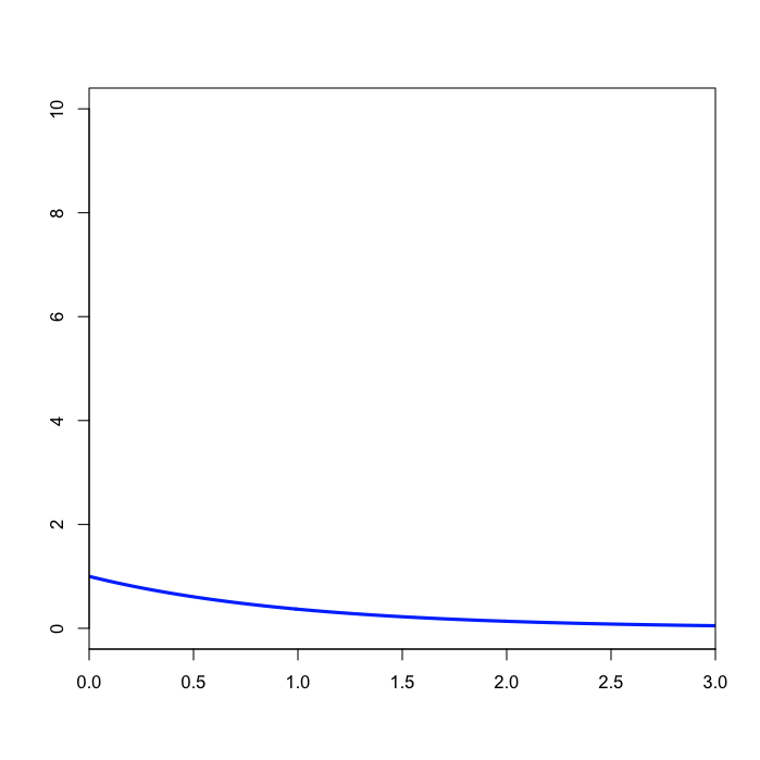
21. What is the mean you expected for alpha based on the prset shapepr=exp(1.0) command in the algaemb.nex file?
answer:
22. What is the posterior mean actually estimated by MrBayes (and presented by Tracer)?
answer:
23. Does the approximated density appear to approach 1/mean at the value alpha=0.0?
answer:
24. What is the posterior mean of TL, as reported by Tracer?
answer:
25. What value did you expect based on the prset brlenspr=unconstrained:exp(10) command?
answer:
26. Does the approximated posterior distribution of TL appear to be an exponential distribution?
answer:
27. Does the Gamma(13, 0.1) density appear to match (at least visually) the density of TL as shown by Tracer?
answer:
Create a directory
Use the unix mkdir command to create a directory to play in today:
cd
mkdir mblab
Download and save the data file
Save the contents of the file algaemb.nex to a file in the mblab folder. One easy way to do this is to cd into the mblab folder, then use the curl command (“Copy URL”) to download the file:
cd ~/mblab
curl -O https://gnetum.eeb.uconn.edu/courses/phylogenetics/lab/algaemb.nex
Use nano to look at this file. This is the same 16S data you have used before, but the original file had to be changed to accommodate MrBayes’ eccentricities. While MrBayes does a fair job of reading Nexus files, it chokes on certain constructs. The information about what I had to change in order to get it to work is in a comment at the top of the file (this might be helpful in converting other nexus files to work with MrBayes in the future).
Creating a MRBAYES block
The next step is to set up an MCMC analysis. There are three commands in particular that you will need to know about in order to set up a typical run: lset, prset and mcmc. The command mcmcp is identical to mcmc except that it does not actually start a run. For each of these commands you can obtain online information by typing help followed by the command name: for example, help prset. Start MrBayes interactively by simply typing mb to see how to get help:
mb
This will start MrBayes. At the MrBayes> prompt, type help:
MrBayes> help
To quit MrBayes, type quit at the “MrBayes>” prompt. You will need to quit MrBayes in order to build up the MRBAYES block in your data file.
Create a MRBAYES block at the bottom of your algaemb.nex data file. MrBayes does not have a built-in editor, so you will need to use the nano editor to edit the algaemb.nex data file. Use Ctrl-/, Ctrl-v to jump to the bottom of the file in nano, then add the following at the very bottom of the file to begin creating the MRBAYES block:
begin mrbayes;
    set autoclose=yes seed=12345 swapseed=12345;
end;
Note that I refer to this block as a MRBAYES block (upper case), but the MrBayes program does not care about case, so using mrbayes (lower case) works just fine.
The autoclose=yes statement in the set command tells MrBayes that we will not want to continue the run beyond the 10,000 generations that we will specify. If you leave this out, MrBayes will ask you whether you wish to continue running the chains after the specified number of generations is finished.
The seed=12345 and swapseed=12345 statements will set a seed for your MCMC and swapping between your heated and cold chains, respectively. If you don’t specify a seed, MrBayes will generate random seeds, but you should always explicitly set a seed in order to preserve your ability to later recreate the analysis exactly (or tell others how to recreate it). Note that you could change the seed to be any integer, but we’ll all use 12345 for this lab.
Add subsequent commands (described below) after the set command and before the end; line. Note that commands in MrBayes are (intentionally) similar to those in PAUP, but the differences can be frustrating. For instance, lset ? in PAUP gives you information about the current likelihood settings, but this does not work in MrBayes. Instead, you type help lset. Also, the lset command in MrBayes has many options not present in PAUP*, and vice versa.
Specifying the prior on branch lengths
begin mrbayes;
    set autoclose=yes seed=12345 swapseed=12345;
    prset brlenspr=unconstrained:exp(10.0);
end;
The prset command above specifies that branch lengths are to be unconstrained (i.e. a molecular clock is not assumed) and the prior distribution to be applied to each branch length is an exponential distribution with mean 1/10. Note that the value you specify for unconstrained:exp is the rate, which is the inverse of the mean.
Note that you should only have one mrbayes block in your file at this point. We will be adding to this one mrbayes block as each prior is discussed.
Specifying the prior on the gamma shape parameter
begin mrbayes;
    set autoclose=yes seed=12345 swapseed=12345;
    prset brlenspr=unconstrained:exp(10.0);
    prset shapepr=exp(1.0);
end;
The second prset command specifies an exponential distribution with mean 1.0 for the shape parameter of the gamma distribution we will use to model rate heterogeneity. Note that we have not yet told MrBayes that we wish to assume that substitution rates are variable; we will do that using the lset command below.
Specifying the prior on kappa
begin mrbayes;
    set autoclose=yes seed=12345 swapseed=12345;
    prset brlenspr=unconstrained:exp(10.0);
    prset shapepr=exp(1.0);
    prset tratiopr=beta(1.0,1.0);
end;
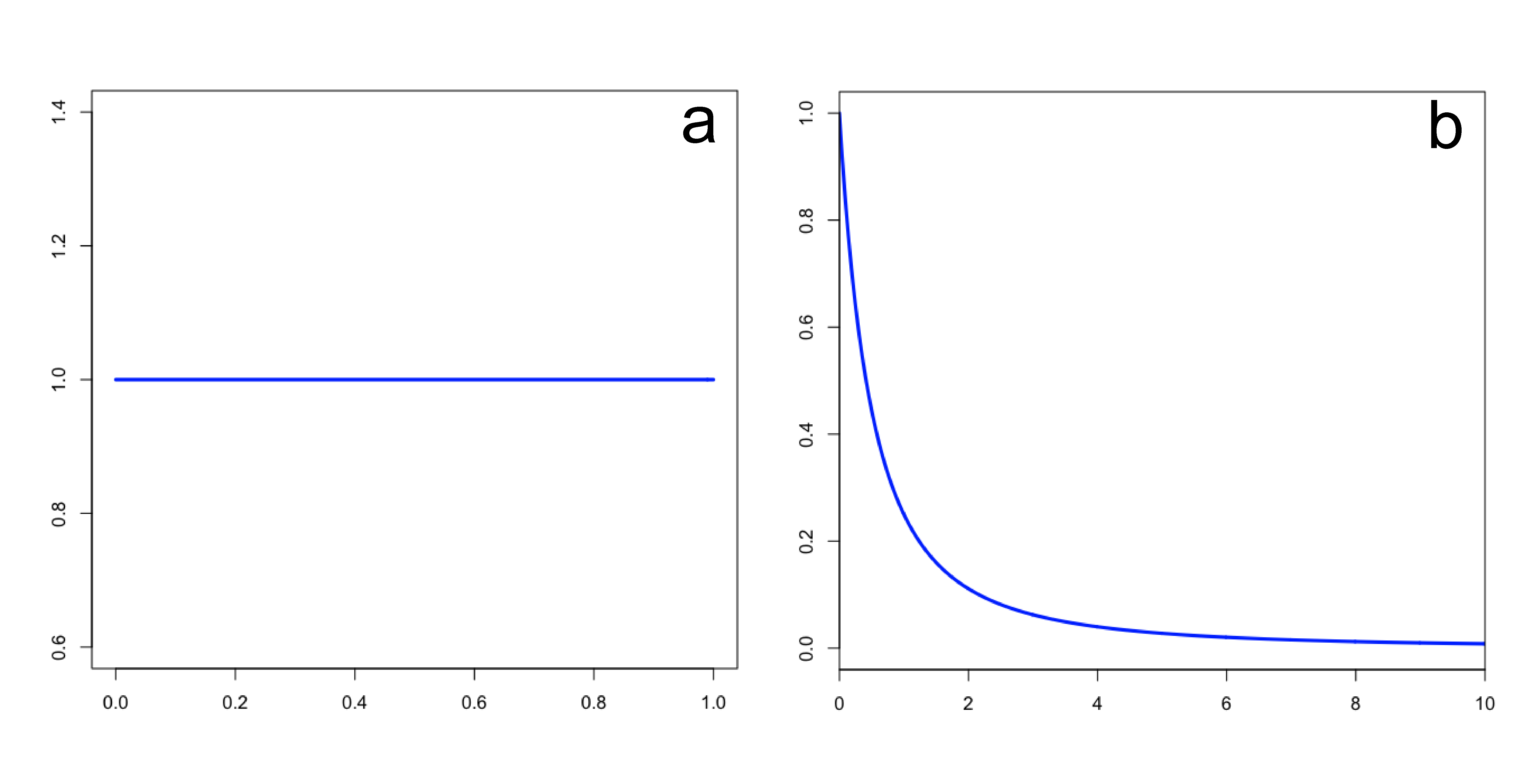
The command above says to use a Beta(1,1) distribution as the prior for the transition/transversion rate ratio. Recall that the kappa parameter is the ratio \(\alpha/\beta\), where \(\alpha\) is the transition rate and \(\beta\) is the transversion rate. Rather than allowing you to place a prior directly on the value of \(\kappa\), MrBayes instead requires you to place a Beta prior on the quantity \(\alpha/(\alpha + \beta)\). The rationale behind this restriction is esoteric.
That said, you might wonder what the Beta(1,1) distribution we’ve specified implies about the distribution of \(\kappa\). Transforming the Beta density into the density of \(\alpha/\beta\) results in the plot on the right. This density for \(\kappa\) is very close, but not identical, to an Exponential(1) distribution. This is known as the Beta Prime distribution, and has support [0, infinity), which is appropriate for a ratio such as \(\kappa\).
Specifying a prior on base frequencies
begin mrbayes;
    set autoclose=yes seed=12345 swapseed=12345;
    prset brlenspr=unconstrained:exp(10.0);
    prset shapepr=exp(1.0);
    prset tratiopr=beta(1.0,1.0);
    prset statefreqpr=dirichlet(1.0,1.0,1.0,1.0);
end;
The above command states that a flat Dirichlet distribution is to be used for base frequencies. The Dirichlet distribution is like the Beta distribution, except that it is applicable to combinations of parameters. Like the Beta distribution, the distribution is symmetrical if all the parameters of the distribution are equal, and the distribution is flat if all the parameters of the distribution are equal to 1.0. Using the command above specifies a flat Dirichlet prior, which says that any combination of base frequencies will be given equal prior weight. This means that (0.01, 0.99, 0.0, 0.0) has the same probability density, a priori, as (0.25, 0.25, 0.25, 0.25). If you wanted base frequencies to not stray much from (0.25, 0.25, 0.25, 0.25), you could specify, say, statefreqpr=dirichlet(100,100,100,100) instead.
This applet lets you experiment with a Dirichlet prior on base frequencies. Try spinning it around by dragging your mouse left to right (or right to left), and try changing from a Dirichlet(1,1,1,1) to a Dirichlet(100,100,100,100) to see the effect.
The lset command
begin mrbayes;
    set autoclose=yes seed=12345 swapseed=12345;
    prset brlenspr=unconstrained:exp(10.0);
    prset shapepr=exp(1.0);
    prset tratiopr=beta(1.0,1.0);
    prset statefreqpr=dirichlet(1.0,1.0,1.0,1.0);
    lset nst=2 rates=gamma ngammacat=4;
end;
We are finished setting priors now, so the lset command above finishes our specification of the model by telling MrBayes that we would like a 2-parameter substitution matrix (i.e. the rate matrix has only two substitution rates, the transition rate and the transversion rate). It also specifies that we would like rates to vary across sites according to a gamma distribution with 4 categories.
Specifying MCMC options
begin mrbayes;
    set autoclose=yes seed=12345 swapseed=12345;
    prset brlenspr=unconstrained:exp(10.0);
    prset shapepr=exp(1.0);
    prset tratiopr=beta(1.0,1.0);
    prset statefreqpr=dirichlet(1.0,1.0,1.0,1.0);
    lset nst=2 rates=gamma ngammacat=4;
    mcmcp ngen=10000 samplefreq=10 printfreq=100 nruns=1 nchains=3 savebrlens=yes;
end;
The mcmcp command above specifies most of the remaining details of the analysis.
ngen=10000 tells MrBayes that its MCMC robots should each take 10,000 steps. You should ordinarily use much larger values for ngen than this (the default is 1 million steps). We’re keeping it small here because we do not have a lot of time and the purpose of this lab is to learn how to use MrBayes, not produce a publishable result.
samplefreq=10 says to only save parameter values and the tree topology every 10 steps. This gives the robot a chance to wander a little bit away from its last known location before peeking at it again.
printfreq=100 says that we would like a progress report every 100 steps.
nruns=1 says to just do one independent run. MrBayes performs two separate analyses by default.
nchains=3 says that we would like to have 2 heated chains running in addition to the cold chain. MrBayes uses 4 chains by default.
Finally, savebrlens=yes tells MrBayes that we would like it to save branch lengths when it saves the sampled tree topologies.
Specifying an outgroup
begin mrbayes;
    set autoclose=yes seed=12345 swapseed=12345;
    prset brlenspr=unconstrained:exp(10.0);
    prset shapepr=exp(1.0);
    prset tratiopr=beta(1.0,1.0);
    prset statefreqpr=dirichlet(1.0,1.0,1.0,1.0);
    lset nst=2 rates=gamma ngammacat=4;
    mcmcp ngen=10000 samplefreq=10 printfreq=100 nruns=1 nchains=3 savebrlens=yes;
    outgroup Anacystis_nidulans;
end;
The outgroup command merely affects the display of trees. It says we want trees to be rooted between the taxon Anacystis nidulans and everything else.
Running MrBayes and interpreting the results
Now save the file and start MrBayes (from within the mblab directory) by typing
mb
Once it starts, type the following at the MrBayes> prompt
exe algaemb.nex
Alternatively, you could both start MrBayes and execute the data file like this:
mb -i algaemb.nex
The -i tells MrBayes to wait for further commands (i.e. be interactive).
Once MrBayes has finished executing the data file, type the following at the MrBayes> prompt:
mcmc
This command starts the run. While MrBayes runs, it shows one-line progress reports. The first column is the iteration (generation) number. The next three columns show the log-likelihoods of the separate chains that are running, with the cold chain indicated by square brackets rather than parentheses. The last complete column is a prediction of the time remaining until the run completes. The columns consisting of only -- are simply separators, they have no meaning.
Do you see evidence that the 3 chains are swapping with each other?
The section entitled Chain swap information: reports the number of times each of the three chains attempted to swap with one of the other chains (three values in lower left, below the main diagonal) and the proportion of time such attempts were successful (three values in upper right, above the main diagonal).
When the run has finished, MrBayes will report (in the section entitled Acceptance rates for the moves in the "cold" chain:) various statistics about the run, such as the percentage of time it was able to accept proposed changes of various sorts. These percentages should, ideally, all be between about 20% and 50%, but as long as they are not extreme (e.g. 1% or 99%) then things went well. Even if there are low acceptance rates for some proposal types, this may not be important if there are other proposal types that operate on the same parameters. For example, note that ExtSPR, ExtTBR, NNI and PrsSPR all operate on Tau, which is the tree topology. As long as these proposals are collectively effective, the fact that one of them is accepting at a very low rate is not of concern.
Below is the acceptance information for my run:
Acceptance rates for the moves in the "cold" chain:
   With prob.   (last 100)   chain accepted proposals by move
     35.2 %     ( 36 %)     Dirichlet(Tratio)
      NA           NA       Dirichlet(Pi)
      NA           NA       Slider(Pi)
     51.5 %     ( 51 %)     Multiplier(Alpha)
      7.0 %     ( 10 %)     ExtSPR(Tau,V)
      6.0 %     (  5 %)     ExtTBR(Tau,V)
     10.6 %     (  9 %)     NNI(Tau,V)
     10.6 %     (  7 %)     ParsSPR(Tau,V)
     49.4 %     ( 44 %)     Multiplier(V)
     28.5 %     ( 39 %)     Nodeslider(V)
     17.6 %     ( 15 %)     TLMultiplier(V)
In the above table, 51.5% of proposals to change the gamma shape parameter (denoted Alpha by MrBayes) were accepted. This makes it sounds as if the gamma shape parameter was changed quite often, but to get the full picture, you need to scroll up to the beginning of the output and examine this section:
The MCMC sampler will use the following moves:
   With prob.  Chain will use move
      1.89 %   Dirichlet(Tratio)
      0.94 %   Dirichlet(Pi)
      0.94 %   Slider(Pi)
      1.89 %   Multiplier(Alpha)
      9.43 %   ExtSPR(Tau,V)
      9.43 %   ExtTBR(Tau,V)
      9.43 %   NNI(Tau,V)
      9.43 %   ParsSPR(Tau,V)
     37.74 %   Multiplier(V)
     13.21 %   Nodeslider(V)
      5.66 %   TLMultiplier(V)
This says that an attempt to change the gamma shape parameter will only be made in fewer than 2% of the iterations.
The fact that MrBayes modified the gamma shape parameter only about 1% of the time brings up a couple of important points. First, in each iteration, MrBayes chooses a move (i.e. proposal) at random to try. Each move is associated with a “Rel. prob.” (relative probability).
Type showmoves to show the list of moves that were used in this particular analysis:
Moves that will be used by MCMC sampler (rel. proposal prob. > 0.0):

  1 -- Move        = Dirichlet(Tratio)
       Type        = Dirichlet proposal
       Parameter   = Tratio [param. 1] (Transition and transversion rates)
       Tuningparam = alpha (Dirichlet parameter)
             alpha = 49.502
       Targetrate  = 0.250
       Rel. prob.  = 1.0

  2 -- Move        = Dirichlet(Pi)
       Type        = Dirichlet proposal
       Parameter   = Pi [param. 2] (Stationary state frequencies)
       Tuningparam = alpha (Dirichlet parameter)
             alpha = 100.000  [chain 1]
                     101.005  [chain 2]
                     100.000  [chain 3]
       Targetrate  = 0.250
       Rel. prob.  = 0.5

  3 -- Move        = Slider(Pi)
       Type        = Sliding window
       Parameter   = Pi [param. 2] (Stationary state frequencies)
       Tuningparam = delta (Sliding window size)
             delta = 0.200  [chain 1]
                     0.202  [chain 2]
                     0.200  [chain 3]
       Targetrate  = 0.250
       Rel. prob.  = 0.5

  4 -- Move        = Multiplier(Alpha)
       Type        = Multiplier
       Parameter   = Alpha [param. 3] (Shape of scaled gamma distribution of site rates)
       Tuningparam = lambda (Multiplier tuning parameter)
            lambda = 0.819
       Targetrate  = 0.250
       Rel. prob.  = 1.0

  5 -- Move        = ExtSPR(Tau,V)
       Type        = Extending SPR
       Parameters  = Tau [param. 5] (Topology)
                     V [param. 6] (Branch lengths)
       Tuningparam = p_ext (Extension probability)
                     lambda (Multiplier tuning parameter)
             p_ext = 0.500
            lambda = 0.098
       Rel. prob.  = 5.0

  6 -- Move        = ExtTBR(Tau,V)
       Type        = Extending TBR
       Parameters  = Tau [param. 5] (Topology)
                     V [param. 6] (Branch lengths)
       Tuningparam = p_ext (Extension probability)
                     lambda (Multiplier tuning parameter)
             p_ext = 0.500
            lambda = 0.098
       Rel. prob.  = 5.0

  7 -- Move        = NNI(Tau,V)
       Type        = NNI move
       Parameters  = Tau [param. 5] (Topology)
                     V [param. 6] (Branch lengths)
       Rel. prob.  = 5.0

  8 -- Move        = ParsSPR(Tau,V)
       Type        = Parsimony-biased SPR
       Parameters  = Tau [param. 5] (Topology)
                     V [param. 6] (Branch lengths)
       Tuningparam = warp (parsimony warp factor)
                     r (reweighting probability)
                     v_t (typical branch length)
                     lambda (multiplier tuning parameter)
              warp = 0.100
                 r = 0.050
               v_t = 0.030
            lambda = 0.098
       Rel. prob.  = 5.0

  9 -- Move        = Multiplier(V)
       Type        = Random brlen hit with multiplier
       Parameter   = V [param. 6] (Branch lengths)
       Tuningparam = lambda (Multiplier tuning parameter)
            lambda = 2.007
       Targetrate  = 0.250
       Rel. prob.  = 20.0

 10 -- Move        = Nodeslider(V)
       Type        = Node slider (uniform on possible positions)
       Parameter   = V [param. 6] (Branch lengths)
       Tuningparam = lambda (Multiplier tuning parameter)
            lambda = 0.191
       Rel. prob.  = 7.0

 11 -- Move        = TLMultiplier(V)
       Type        = Whole treelength hit with multiplier
       Parameter   = V [param. 6] (Branch lengths)
       Tuningparam = lambda (Multiplier tuning parameter)
            lambda = 1.319  [chain 1]
                     1.345  [chain 2]
                     1.345  [chain 3]
       Targetrate  = 0.250
       Rel. prob.  = 3.0
Summing the 11 relative probabilities yields 1 + 0.5 + 0.5 + 1 + 5 + 5 + 5 + 5 + 20 + 7 + 3 = 53. To get the probability of using one of these moves in any particular iteration, MrBayes divides the relative probability for the move by this sum. Thus, move 4, whose job is to update the gamma shape parameter (called Alpha by MrBayes) will be chosen with probability 1/53 = 0.01886792. This is where the “1.89 % Multiplier(Alpha)” line comes from in the move probability table spit out just before the run started.
Second, note that MrBayes places a lot of emphasis on modifying the tree topology and branch lengths (in this case 100*(5+5+5+5+20+7+3)/53 = 94% of proposals), but puts little effort (in this case only 6%) into updating other model parameters. You can change the percent effort for a particular move using the propset command. For example, to increase the effort devoted to updating the gamma shape parameter, you could (but don’t do this now!) issue the following command either at the MrBayes prompt or in a MRBAYES block:
propset Multiplier(Alpha)$prob=10 [*** don't type this ***]
This would change the relative probability of the “Multiplier(Alpha)” move from its default value 1 to the value you specified (10). You can also change tuning parameters for moves using the propset command. Before doing that, however, we need to see if the boldness of any moves needs to be changed.
The sump command
MrBayes saves information in several files. Only two of these will concern us today. One of them will be called algaemb.nex.p. This is the file in which the sampled parameter values were saved. This file is saved as a tab-delimited text file so it is possible to read it into a variety of programs that can be used for summarization or plotting. We will examine this file graphically in a moment, but first let’s get MrBayes to summarize its contents for us.
At the MrBayes prompt, type the command sump. This will generate a crude graph showing the log-likelihood as a function of time. Note that the log-likelihood bounces around between -3183 and -3176. The fact that it is bouncing around is a sign that the MCMC simulation is mixing well.
Below the graph, MrBayes provides the arithmetic mean and harmonic mean of the marginal likelihood. The harmonic mean has been often used in estimating Bayes factors, which are in turn useful for deciding which among different models fits the data best on average. You heard in lecture that this value can be used for Bayesian model selection, but you also got some dire warnings about Bayes factors calculated using the Harmonic Mean method. There are much more accurate methods for estimating marginal likelihoods than the harmonic mean method. I’m not aware of any use for the Arithmetic Mean.
The table at the end is quite useful. It shows the (marginal) posterior mean, median, variance and 95% credible interval for each parameter in your model based on the samples taken during the run. The credible interval shows the range of values of a parameter that account for the middle 95% of its marginal posterior distribution. If the credible interval for kappa is 3.9 to 5.9, then you can say that there is a 95% chance that kappa is between 3.9 and 5.9 given your data and the assumed model. The parameter TL represents the sum of all the branch lengths. Rather than report every branch length individually, MrBayes just keeps track of their sum.
Look at the output of the sump command and answer these questions:
The ESS (Effective Sample Size) tells you something about autocorrelation in your sample. Imagine drawing 1 variate from a Normal distribution and then copying that value 1000 times. You have, nominally, a sample of 1000 values, but they are all copies of just 1 independent draw. In this case, the ESS would be 1, not 1000. Now imagine drawing 10 values from a Normal distribution and copying each of them 100 times. This time, the ESS would be 10 even though the sample size is 1000. Tracer measures the autocorrelation (how correlated each sampled value is to the previous one, and the one before that, and so on, in order to measure the ESS of your sample. It shows (what it considers) low ESS values in yellow and really low ESS values in red. You should run your MCMC analysis long enough that the ESS is not yellow or red for at least the parameters you care most about (and, ideally, all of the ESS should be out of the danger zone).
The sumt command
Now type the command sumt. This will summarize the trees that have been saved in the file algaemb.nex.t.
The output of this command includes a bipartition (split) table, showing marginal posterior probabilities for every split found in any tree sampled during the run. After the bipartition table is shown a majority-rule consensus tree (labeled “Clade credibility values”) containing all splits that had marginal posterior probability 0.5 or above.
If you chose to save branch lengths (and we did), MrBayes shows a second tree (labeled Phylogram) in which each branch is displayed in such a way that branch lengths are proportional to their posterior mean. MrBayes keeps a running sum of the branch lengths for particular splits it finds in trees as it reads the file algaemb.nex.t. Before displaying this tree, it divides the sum for each split by the total number of times it encountered the split to get a simple average branch length for each split. It then draws the tree so that branch lengths are proportional to these mean branch lengths.
Finally, the last thing the sumt command does is tell you how many tree topologies are in credible sets of various sizes. For example, in my run, it said that the 99% credible set contained 16 trees. What does this tell us? MrBayes orders tree topologies from most frequent to least frequent (where frequency refers to the number of times they appear in algaemb.nex.t). To construct the 99% credible set of trees, it begins by adding the most frequent tree to the set. If that tree accounts for 99% or more of the marginal posterior probability (i.e. at least 99% of all the trees in the algaemb.nex.t file have this topology), then MrBayes would say that the 99% credible set contains 1 tree. If the most frequent tree topology was not that frequent, then MrBayes would add the next most frequent tree topology to the set. If the combined marginal posterior probability of both trees was at least 0.99, it would say that the 99% credible set contains 2 trees. In my case, it had to add the top 16 trees to get the total posterior probability up to 99%.
Type quit (or just q), to quit MrBayes now.
Using Tracer to summarize MCMC results
The Java program Tracer is very useful for summarizing the results of Bayesian phylogenetic analyses. Tracer was written to accompany the program Beast, but it works well with the output file produced by MrBayes as well. This lab was written using Tracer version 1.7.1, and works with version 1.7.2.
To use Tracer on your own computer to view files created on the cluster, you need to get the file on the cluster downloaded to your laptop. Download the file algaemb.nex.p (using Cyberduck, FileZilla, Fugu, scp, or whatever has been working).
After starting Tracer, choose File > Import Trace File… to choose a parameter sample file to display (you can also do this by clicking the + button under the list of trace files in the upper left corner of the main window). Select the algaemb.nex.p file in your working folder, then click the Open button to read it.
You should now see 9 rows of values in the table labeled Traces on the left side of the main window. The first row (LnL) is selected by default, and Tracer shows a histogram of log-likelihood values on the right, with summary statistics above the histogram.
A histogram is perhaps not the most useful plot to make with the LnL values. Click the Trace tab to see a trace plot (plot of the log-likelihood through time).
Tracer determines the burn-in period using an undocumented algorithm. You may wish to be more conservative than Tracer. Opinions vary about burn-in. Some Bayesians feel it is important to exclude the first few samples because it is obvious that the chains have not reached stationarity at this point. Other Bayesians feel that if you are worried about the effect of the earliest samples, then you definitely have not run your chains long enough! You might be interested in reading Charlie Geyer’s rant on burn-in some time.
Our MrBayes run was just to learn how to run MrBayes and not to do a serious analysis. The fact that a longer run is needed is indicated by all the ESS values shown in red in the Traces panel. Tracer shows an ESS in red if it is less than 200, which it treats as the minimal reasonable effective sample size.
Click the Estimates tab again at the top, then click the row labeled kappa on the left.
Click the row labeled alpha on the left. This is the shape parameter of the gamma distribution governing rates across sites.
Click on the row labeled TL on the left (the Tree Length).
Scatterplots of pairs of parameters
Note that Tracer lets you easily create scatterplots of combinations of parameters. Simply select two parameters (you will have to hold down the Ctrl or Cmd key to select multiple items) and then click on the “Joint-Marginal” tab.
Marginal densities
Try selecting all four base frequencies and then clicking the “Marginal Density” tab. This will show (estimated) marginal probability density plots for all four frequencies at once. Note that KDE is selected underneath the plot in the Display drop-down list. KDE stands for “Kernel Density Estimation” and represents a common non-parametric method for smoothing histograms into estimates of probabilty density functions.
Running MrBayes with no data
Running a Bayesian MCMC program without data is a good way to make sure you know what priors you are actually placing on the quantities of interest. It provides an easy sanity check to ensure that the priors were set the way you thought, and a way to see induced priors for quantities for which you could not explicitly assign a prior distribution, such as tree length (TL) and particular splits of interest.
If there is no information in the data, the posterior distribution equals the prior distribution. An MCMC analysis in this case provides an approximation of the prior. MrBayes makes it easy to run the MCMC analysis without data. (For programs that don’t make it easy, simply create a data set containing just one site for which each taxon has missing data.)
Start by moving the output from the earlier run of the algaemb.nex data file to a directory named saved:
mkdir saved
mv algaemb.nex.* saved
The above command will leave the data file algaemb.nex behind, but move files with names based on the data file but which append other characters to the filename, such as algaemb.nex.p and algaemb.nex.t into the newly-created directory saved.
If the only file remaining in the mblab directory is the algaemb.nex data file, type the following to start the data-free analysis:
mb -i algaemb.nex
MrBayes> mcmc data=no ngen=1000000 samplefreq=100
Note that I have increased the number of generations to 1 million because the run will go very fast. Sampling every 100th generation will give us a sample of size 10000 to work with.
Checking the shape parameter prior
On your local laptop, rename algaemb.nex.p to something like algaemb-posterior.p, then download the file algaemb.nex.p to your laptop, renaming it algaemb-prior.p. Open algaemb-prior.p in Tracer. Look first at the histogram of alpha, the shape parameter of the gamma distribution.
Checking the branch length prior
Now look at the histogram of TL, the tree length.
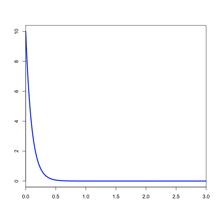
The second and third questions are a bit tricky, so I’ll just give you the explanation. Please make sure this explanation makes sense to you, however, and ask us to explain further if it doesn’t make sense. We told MrBayes to place an exponential prior with mean 0.1 on each branch. There are 13 branches in a 8-taxon, unrooted tree. Thus, 13 times 0.1 equals 1.3, which should be close to the posterior mean you obtained for TL. That part is fairly straightforward.
The marginal distribution of TL does not look at all like an exponential distribution, despite the fact that TL should be the sum of 13 exponential distributions. It turns out that the sum of \(n\) independent Exponential(\(\lambda\)) distributions is a Gamma(\(n\), \(1/\lambda\)) distribution. In our case the tree length distribution is a sum of 13 independent Exponential(10) distributions, which equals a Gamma(13, 0.1) distribution. Such a Gamma distribution would have a mean of (13)(0.1) = 1.3 and a variance of (13)(.1)(.1) = 0.13.
To visualize this, fire up RStudio and type the following command:
curve(dgamma(theta, shape=13, scale=0.1), from=0, to=2, xname="theta")