RevBayes Morphology Lab

Up to the Phylogenetics main page

Goals

This lab exercise will show how to analyze discrete morphological data using RevBayes. We will be using RevBayes v1.1.1 on the cluster in this lab.

This lab exercise is adapted from the tutorial entitled Discrete morphology - Tree Inference on the RevBayes web site.

Answer template

Here is a template in which to save your answers to the questions.

1. Is brlen_lambda a parameter or a hyperparameter in this model?
answer:

2. What is the posterior mean tree length for the M2 model using the combined parameter samples from both runs?
answer:

3. How many total characters are in this data matrix?
answer:

4. How many characters in this data matrix are variable?
answer:

5. Do you expect estimated tree length to increase or decrease if we condition on variability? Briefly explain your reasoning.
answer:

6. What is the posterior mean tree length for the Mkv model?
answer:

7. Did the Mkv model have the effect you expected?
answer:

8. In lecture, you were shown simulation results that suggested that estimates of edge lengths would be severely wrong unless the model conditioned on variability. Why did it make so little difference here?
answer:

9. What do the values in the categ_means vector represent? Note: do not say these are the category means, which you can deduce from the name of the variable. Instead, state how these values are used in the likelihood calculation.
answer:

10. What do the values in the categ_probs vector represent?
answer:

11. Of the 3 models, which fits substantially worse than the others?
answer:

12. Does allowing heterogeneity in state frequency provide substantially better fit than simply assuming equal state frequencies?
answer:

13. If you were preparing to publish a paper relating to these analyses, you probably would not want to depend on eyeballing box plots of the likelihood in Tracer. What quantity would you estimate to convince reviewers that one of these models fits the data much worse than the other two?
answer:

Getting started

Login to your account on the Health Center (Xanadu) cluster, then issue

srun --qos=mcbstudent --partition=mcbstudent --mem=5G --pty bash

to start a session on a node that is not currently running jobs.

Important The --mem=5G part is important for this lab, as RevBayes uses more than the default amount (128 MB) of memory sometimes.

Create a directory

Use the unix mkdir command to create a directory to play in today:

cd
mkdir morphlab

Load the RevBayes module

You will need to load the RevBayes/1.1.1 module in order to use RevBayes:

module load RevBayes/1.1.1

You can now type either RevBayes or just rb to start the program.

Download and save the data file

Use the curl command (“Copy URL”) to download the data file for this tutorial from the RevBayes web site:

cd ~/morphlab
curl -O https://revbayes.github.io/tutorials/morph_tree/data/bears.nex

Creating a RevBayes script

Create a RevBayes script to carry out an MCMC analysis using the simplest 2-state Mk model.

Use nano to create a file (I’m assuming you are currently in the ~/morphlab folder where your data file is located.

nano mk.Rev

The scripts we will create today will end up being almost identical to the files mcmc_mk.Rev, mcmc_mkv.Rev, and mcmc_mkv_discretized.Rev (written by April M. Wright, Michael J. Landis, and Sebastian Höhna) from the Discrete morphology tutorial.

Read the data file

Enter the following text and then save the file:

###############
# Data matrix #
###############

morpho <- readDiscreteCharacterData("bears.nex")
taxa <- morpho.names()
num_taxa <- taxa.size()
num_branches <- 2 * num_taxa - 2

moves    = VectorMoves()
monitors = VectorMonitors()

Add a tree model

The tree model specifies a prior for tree topology as well as a prior for edge lengths. We will also use this section to specify proposals (called moves in RevBayes) for modifying both tree topology and edge lengths.

##############
# Tree model #
##############

brlen_lambda ~ dnExponential(0.1)
moves.append( mvScale(brlen_lambda, weight=2) )

phylogeny ~ dnUniformTopologyBranchLength(taxa, branchLengthDistribution=dnExponential(brlen_lambda))

tree_length := phylogeny.treeLength()

moves.append( mvNNI(phylogeny, weight=num_branches/2.0) )
moves.append( mvSPR(phylogeny, weight=num_branches/10.0) )
moves.append( mvBranchLengthScale(phylogeny, weight=num_branches) )

Is brlen_lambda a parameter or a hyperparameter in this model?

Create a substitution model

Append the following to your script to specify a substitution model:

######################
# Substitution Model #
######################

Q <- fnJC(2)

gamma_shape ~ dnExponential(0.01)
moves.append( mvScale(gamma_shape,lambda=1, weight=2.0) )

gamma_rate := gamma_shape
gamma_rates := fnDiscretizeGamma( gamma_shape, gamma_rate, 4 )

This tells RevBayes to create a Jukes-Cantor instantaneous rate matrix with 2 states (also known as a 2-state Mk, or M2, model) and store it in the variable Q.

The PhyloCTMC node puts everything together

#############
# PhyloCTMC #
#############

# Specify the probability distribution of the data given the model
likelihood ~ dnPhyloCTMC(tree=phylogeny, siteRates=gamma_rates, Q=Q, type="Standard")

# Attach the data
likelihood.clamp(morpho)

mymodel = model(phylogeny)

Ready for MCMC

We’ve now completely specified the model, so all that’s left is to create some monitors so that results are saved and set up the mcmc command.

#################
# MCMC Analysis #
#################

# Add monitors
monitors.append( mnModel(filename="output/mk.log", printgen=10) )
monitors.append( mnFile(filename="output/mk.trees", printgen=10, phylogeny) )
monitors.append( mnScreen(printgen=100) )

# Start the MCMC analsis
mymcmc = mcmc(mymodel, monitors, moves, nruns=2, combine="mixed")
mymcmc.burnin(generations=2000, tuningInterval=200)
mymcmc.run(generations=20000)

# Check the performance of the moves (also known as operators)
mymcmc.operatorSummary()

# Read in the tree trace and construct the consensus tree tree
trace = readTreeTrace("output/mk.trees", treetype="non-clock")
trace.setBurnin(0.25)

# Summarize tree trace and the consensus tree to file
mapTree(trace, file="output/mk.map.tre")
consensusTree(trace, file="output/mk.majrule.tre")

# Quit RevBayes
quit()

Run your file in RevBayes now:

rb mk.Rev

Note that it saved the output in a directory named output, which it generated because you included output/ in each of the output file paths.

Open the files mk_run_1.log and mk_run_2.log in Tracer and, after selecting both files in the Trace Files section, click the Marginal Density tab and look through density plots for the Posterior, Likelihood, Prior, brlen_lambda, gamma_shape, and tree_length. The two independent runs should have yielded very similar results.

Now remove the two independent run log files from Tracer’s list (by selecting each of them and pressing the - button below the list), then load the combined log file mk.log.

What is the posterior mean tree length for the M2 model using the combined parameter samples from both runs?

Conditioning on variability

We will now see what effect conditioning on variability makes. When the Mk model conditions on variability, it is denoted the Mkv model.

Use the exclude (exclude character) command in PAUP* to determine how many variable characters are present in the data set we are using:

module load paup/4.0a-166
paup bears.nex
paup> exclude constant
paup> quit

How many total characters are in this data matrix?

How many characters in this data matrix are variable?

Do you expect estimated tree length to increase or decrease if we condition on variability? Briefly explain your reasoning.

Start by copying your mk.Rev script, naming the copy mkv.Rev:

cp mk.Rev mkv.Rev

Now open mkv.Rev in nano and change all the output file names as follows:

old output file	new output file
output/mk.log	output/mkv.log
output/mk.trees	output/mkv.trees
output/mk.map.tre	output/mkv.map.tre
output/mk.majrule.tre	output/mkv.majrule.tre

Note that there are only 4 file names listed here but there are 5 lines you need to change and all are in the MCMC Analysis section.

The only change we need to make to cause RevBayes to condition on variability is to add coding=”variable” to our PhyloCTMC call:

#############
# PhyloCTMC #
#############

# Specify the probability distribution of the data given the model
likelihood ~ dnPhyloCTMC(tree=phylogeny, siteRates=gamma_rates, Q=Q, type="Standard", coding="variable")

Rerun RevBayes using the mkv.Rev script:

rb mkv.Rev

Load the output/mkv.log file into Tracer

What is the posterior mean tree length for the Mkv model?

Did the Mkv model have the effect you expected?

In lecture, you were shown simulation results that suggested that estimates of edge lengths would be severely wrong unless the model conditioned on variability. Why did it make so little difference here?

Beta-distributed state frequencies

We will try one more modification to our Mk model today. The Mk and Mkv models we’ve used thus far all assume that the forward substitution rate is equal to the reverse substitution rate. This leads to equal equilibrium state frequencies (i.e. \(\pi_0 = \pi_1 = 0.5\)).

We can relax this (as described in lecture) by allowing the likelihood to be a mixture model, thus providing several choices of \(\pi_0\) (and thus \(\pi_1\)) for each character. Some characters will end up giving more weight to smaller values of \(\pi_0\) while other characters will end up giving more weight to larger values.

There are 459 0s and 466 1s in the data matrix, so the overall proportions of 0s and 1s are nearly equal; however, the fraction of 0s for any given character ranges from 0.1 to 0.8, so there is room to allow the frequencies of state 0 and state 1 to vary across characters.

Copy your mkv.Rev script, naming the copy mkvbeta.Rev:

cp mkv.Rev mkvbeta.Rev

Now open mkvbeta.Rev in nano and change all the output file names as follows:

old output file	new output file
output/mkv.log	output/mkvbeta.log
output/mkv.trees	output/mkvbeta.trees
output/mkv.map.tre	output/mkvbeta.map.tre
output/mkv.majrule.tre	output/mkvbeta.majrule.tre

Discretized Beta(2,2) distribution

We will model among-character frequency variation in much the same way we model among-character rate variation, using a discretized probability distribution. The main difference is that frequencies are constrained to the part of the real number line between 0.0 and 1.0, so we will use a discrete Beta distribution rather than the discrete Gamma distribution used for modeling rate heterogeneity.

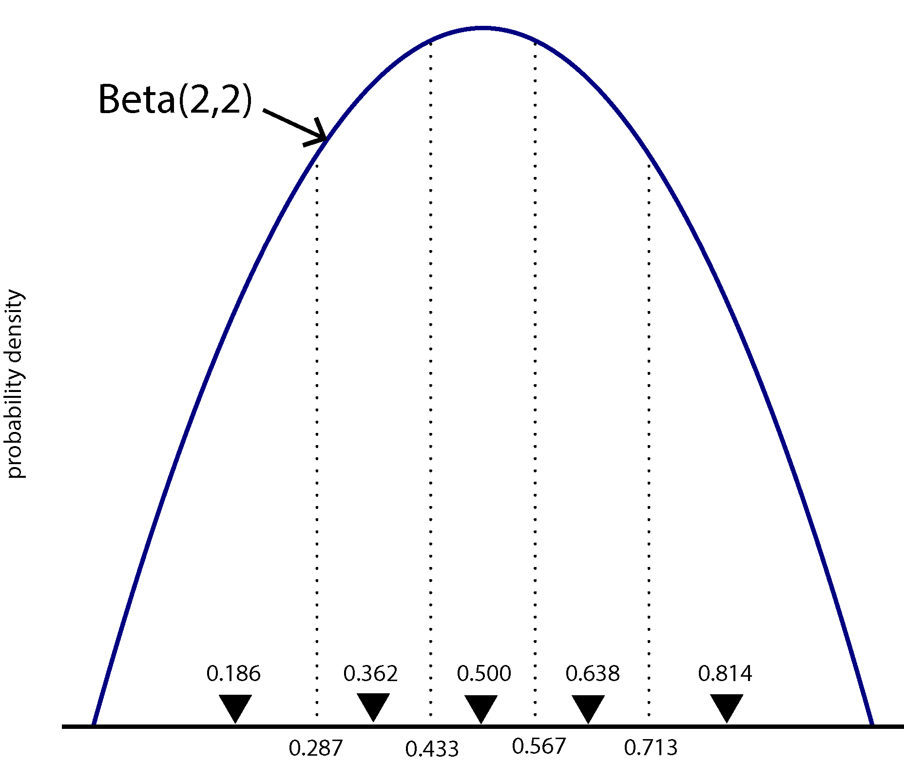
The figure above shows a Beta(2,2) density divided into 5 equal-area categories, with the mean of each category shown using a downward-pointing filled triangle. The likelihood for one character will be calculated using 5 different rate matrices, each using \(\pi_0\) from a different category mean. Each component of the mixture will have probability 0.2, as that is the area under the Beta density curve for each category (assuming there are 5 categories).

Thus, we need 5 different Q matrices in our model, one for each category, so Q in our script will now be a vector of rate matrices rather than a single rate matrix. The shape parameter beta_shape used to determine the symmetric Beta(beta_shape,beta_shape) distribution used will be allowed to vary during the MCMC run, so the 5 Q matrices must be recalculated each time beta_shape changes. This is accomplished by making each element of the Q vector a deterministic node. The recalculation of each rate matrix is accomplished by the fnDiscretizeBeta function (just as the fnDiscretizeGamma function handles recalculation of relative rates for the discrete gamma rate heterogeneity model as the gamma_shape parameter changes).

Here is the entire Substitution Model section. Everything here has changed except for the last 5 lines, all but the last of which are related to rate heterogeneity and are the same lines we used for the Mkv model.

######################
# Substitution Model #
######################

# Specify number of categories to create
num_beta_cats = 5

# Create the parameter that will determine the shape of the Beta distribution
beta_shape ~ dnLognormal( 1.0, sd=1.0 )
moves.append( mvScale(beta_shape, lambda=1, weight=5.0 ) )

# Calculate means of each category
beta_shape.setValue(2.0);
categ_means := fnDiscretizeBeta(beta_shape, beta_shape, num_beta_cats)
print("categ_means = ",categ_means)

# Create vector of Q matrices
for (i in 1:num_beta_cats)
{
    Q[i] := fnF81(simplex(categ_means[i], abs(1-categ_means[i])))
}

categ_probs <- simplex( rep(1,num_beta_cats) )
print("categ_probs = ",categ_probs)

gamma_shape ~ dnExponential(0.01)
moves.append( mvScale(gamma_shape,lambda=1, weight=2.0) )

gamma_rate := gamma_shape
gamma_rates := fnDiscretizeGamma( gamma_shape, gamma_rate, 4 )

quit()

Before we continue, let’s run this script up to this point so that we can see the output from the two print statements in the code above. We want to stop processing the script right after this block of code, so I’ve inserted a quit() command just after the line that calls fnDiscretizeGamma:

rb mkvbeta.Rev

You can see that we are dividing the Beta distribution into 5 equal chunks (num_beta_cats = 5), providing the beta_shape parameter with a Lognormal prior distribution that heavily favors shapes greater than 1 (84%), which is good because shapes less than 1 create U-shaped Beta density functions that place most weight on the extreme values 0 and 1.

What do the values in the categ_means vector represent? Note: do not say these are the category means, which you can deduce from the name of the variable. Instead, state how these values are used in the likelihood calculation.

Hint: compare them to the figure above. I’ve used the setValue function to ensure that the beta_shape parameter is initially equal to 2 (to correspond with the figure).

What do the values in the categ_probs vector represent?

We need to do one last thing in order for RevBayes to actually use the above substitution model. We need to inform the PhyloCTMC object that we are using a mixture distribution to model the Q matrix. To do this, add siteMatrices=categ_probs to the end of your dnPhyloCTMC function call:

likelihood ~ dnPhyloCTMC(tree=phylogeny, siteRates=gamma_rates, Q=Q, type="Standard", coding="variable", siteMatrices=categ_probs)

Now remove the quit() statement at the end of your Substitution Model section and rerun:

rb mkvbeta.Rev

This will take some time because now RevBayes must calculate each site likelihood 5 times, once for each Q matrix in the mixture distribution. When it is finished, load mk.log, mkv.log, and mkvbeta.log into Tracer and compare their likelihoods using the Estimates and/or Marginal Density tab. Note that you will need to select all three files in the Trace Files section so that you can compare them side-by-side.

Of the 3 models, which fits substantially worse than the others?

Does allowing heterogeneity in state frequency provide substantially better fit than simply assuming equal state frequencies?

If you were preparing to publish a paper relating to these analyses, you probably would not want to depend on eyeballing box plots of the likelihood in Tracer. What quantity would you estimate to convince reviewers that one of these models fits the data much worse than the other two?

What to turn in

Turn in your answers to the thinking questions on the template provided above. Send them to Analisa via Slack.