Homework 5 (MCMC)

Markov chain Monte Carlo (MCMC)

In this homework assignment you will cause a metaphorical “MCMC robot” to move several steps on the landscape shown below. The landscape that your robot will be walking on is the log posterior kernel, which is, at every point along the x-axis, the natural logarithm of the likelihood multiplied by the prior probability density. Because the likelihoood is such a small number, we will keep all the calculations on log scale, in which case the log posterior kernel equals, for every point (edge length), the log prior density plus the log likelihood.

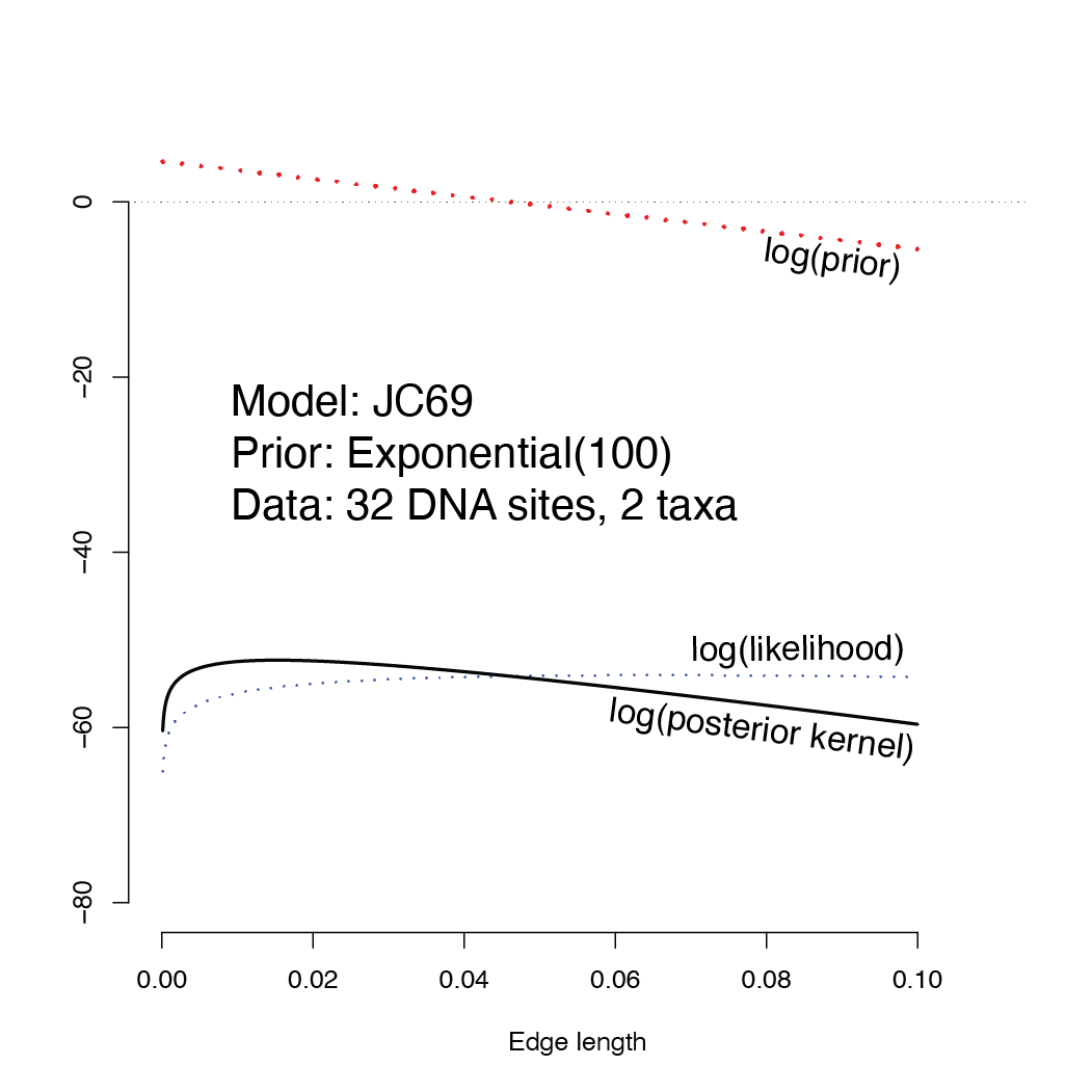
Note how the prior increases toward zero, making the posterior kernel higher than the likelihood for small edge lengths and smaller than the likelihood for larger edge lengths.

You will start your robot at the far right point on this landscape (edge length $v = 0.1$). If your robot is exploring the posterior (kernel), where do you think it will be standing after taking 15 steps? Is it more probable that it will be to the left or to the right of the starting point? You needn’t answer these questions now, but think about them now and see whether your intuition was correct once you’ve done the homework.

How to carry out the calculations

You may use a calculator, spreadsheet program, or a computing language (e.g. R or Python) to do the calculations. I have provided handy helper scripts in both R and Python that do most of the heavy lifting; you need only figure out how to run the script. I highly recommend using either R or Python because calculators are very error-prone (not to mention much more tedious to use). Please ask for help if you are new to R and Python and have trouble getting started. The idea behind these programs is to get you to struggle with the phylogenetics, not the computing tools.

The data

Here is a very small data set that I’ve used in lecture comprising 32 nucleotide sites from the $\psi \eta$-globin pseudogene for gorilla and orangutan. Asterisks indicate the positions of the 2 differences between these sequences.

gorilla   GAAGTCCTTGAGAAATAAACTGCACACACTGG
orangutan GGACTCCTTGAGAAATAAACTGCACACACTGG
           * *

The model

Use the JC69 model for calculating the likelihood, and let the prior for the single parameter $v$ be Exponential(100). The prior probability density for any particular value of $v$ is thus

\[p(v) = 100 e^{-100 v},\]

which means that the log prior density is

\[\log p(v) = \log(100) - 100 v.\]

Important! If you are doing the homework using either a calculator or a spreadsheet program, be careful to use natural logarithms for these calculations. The natural logarithm of 100 is 4.60517 (because $100 = e^{4.60517}$), whereas the common logarithm (base 10) of 100 is 2.0 (because $100 = 10^2$), so use this fact to check to ensure you are using the correct logarithm function on your calculator, python, R, etc.). In most calculators and spreadsheet programs, you must use the ln function to get natural logarithms; the log function calculates the common logarithm. Python and R both use log to mean natural logarithm and use log10 to compute common logarithms.

Starting point

Start your MCMC “robot” at the value $v=0.1$.

Proposal distribution

To propose a new value $v'$ (given current value $v$) for your MCMC robot to consider, use a sliding window of width 0.05 centered over the current value of $v$.

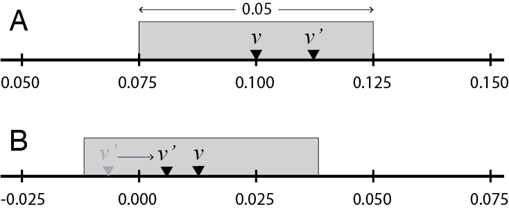
In part A of the figure above, given current value $v = 0.1$ and uniform deviate $u_1 = 0.75$, the proposed new value $v'$ lies 75% of the way across the proposal window (starting from the left end). The proposed value would thus be

\[v' = 0.075 + (0.75)(0.05) = 0.1125.\]

The value 0.075 above is equal to the starting value (0.100) minus half the width of the sliding window (0.025).

Negative proposed values are reflected back into the positive half of the real line. In part B of the figure, the current value is $v = 0.0125$ and the uniform deviate $u_1 = 0.125$, so the proposed new value is

\[v' = −0.0125 + (0.125)(0.05) = −0.00625.\]

This proposed value is negative, and is therefore not a valid value for an edge length, so reflect it back into the valid range by multiplying by -1, yielding $v' = 0.00625.$

What do I turn in?

Please turn in the filled-in worksheet (link to PDF file below) or email/Slack me (paul.lewis@uconn.edu) a photo of the filled in worksheet.

Worksheet in PDF format

Note that some of the rows are already filled in. This will allow you to ensure that you are calculating things correctly. If you get to row 8, for example, and your starting value for that iteration is not 0.06817, then something went wrong in iterations 3-7.

What to do

Each line of the worksheet corresponds to a step taken by your MCMC robot. For each iteration, you will have a starting edge length $v$ (this will be 0.1 for the first iteration) and will need to propose a new value $v'$ using uniform random deviate $u_1$. You will then compute the log of the acceptance ratio $R$ and use uniform random deviate $u_2$ to decide whether to accept the proposed value $v'$ or keep the original value $v$. If you accept the proposed new edge length, then you will use that value as your starting value for the next iteration; if you reject the proposed new edge length, then the next iteration will start with the same value as the current iteration. Note that you will accept $v’$ if $\log(u_2) < \log(R)$ (this is equivalent to asking whether $u_2 < R$).

Helper programs

If you prefer R, use the R helper program. If you prefer Python, use the Python helper program. You do not need to use both!

Python helper

If the python script below is saved as hw5.py, it can be called like this:

python3 hw5.py 0.05

If you don’t have Python 3 installed on your local laptop, you can use Python on the cluster. If the above command does not work, you may need to load the Python module before starting:

module load python

The hw5.py script will compute the log-likelihood, log-prior-density, and log-posterior-kernel for the supplied edge length (i.e. the 0.05 in python3 hw5.py 0.05).

import math, random, sys

# Define a function to calculate the log likelihood given an edge length v
def logLikelihood(v):
    logsame = 2.0*math.log(0.25) + math.log(1.0 + 3.0*math.exp(-4.0*v/3.0))
    logdiff = 2.0*math.log(0.25) + math.log(1.0 - math.exp(-4.0*v/3.0)) 
    return (2.0*logdiff + 30.0*logsame)
    
# Define a function to calculate the log prior given an edge length v
def logPrior(v):
    exponential_rate = 100.0
    return (math.log(exponential_rate) - v*exponential_rate)
    
# Define a function to calculate the log posterior given an edge length v
def logPosteriorKernel(v):
    return (logLikelihood(v) + logPrior(v))
        
# Capture the arguments supplied on the command line (should be just the edge length)       
edge_length = float(sys.argv[1])

# Calculate the log likelihood, log prior, and log posterior kernel
log_likelihood = logLikelihood(edge_length)
log_prior      = logPrior(edge_length)
log_posterior  = logPosteriorKernel(edge_length)

# Output all quantities to the screen
# %12.5f says to format the number with 5 decimal places in a field of width 12
# print is a function that outputs its argument to the console
print('v                     = %12.5f' % edge_length)
print('log(likelihood)       = %12.5f' % log_likelihood)
print('log(prior)            = %12.5f' % log_prior)
print('log(posterior kernel) = %12.5f' % log_posterior)

Thus, the hw5.py program will calculate every quantity you need except for the proposed edge length. The uniform random variates you need to choose the proposed edge length given the current edge length are provided (so that you will get the same answer as me, making it much easier for me to grade!).

Even though hw5.py spits out the log-likelihood and log-prior, the only quantity you need is the log-posterior-kernel. The posterior kernel is the height of the “landscape” that the “robot” is exploring.

Note that $\log(R)$ equals the log-posterior-kernel of the proposed edge length minus the log-posterior-kernel of the current point. The value of $\log(R)$ will be negative if the “robot” is proposing to go downhill and will be positive if it is proposing to go uphill.

R helper

If the R script below is saved as hw5.R, it can be called like this:

Rscript hw5.R 0.05

If you don’t have R installed on your local laptop, you can use R on the cluster. If the above command does not work, you may need to start an interative session:

srun -n 1 -N 1 -p general --pty bash

and then load the R module before starting:

module load r

The hw5.R script will compute the log-likelihood, log-prior-density, and log-posterior-kernel for the supplied edge length (i.e. the 0.05 in Rsxript hw5.R 0.05).

# Define a function to calculate the log likelihood given an edge length v
logLikelihood <- function(v) {
    logsame <- 2.0*log(0.25) + log(1.0 + 3.0*exp(-4.0*v/3.0))
    logdiff <- 2.0*log(0.25) + log(1.0 - exp(-4.0*v/3.0)) 
    return (2.0*logdiff + 30.0*logsame)
    }
    
# Define a function to calculate the log prior given an edge length v
logPrior <- function(v) {
    exponential_rate <- 100.0
    return (log(exponential_rate) - v*exponential_rate)
}
    
# Define a function to calculate the log posterior given an edge length v
logPosteriorKernel <- function(v) {
    return (logLikelihood(v) + logPrior(v))
}

# Capture the arguments supplied on the command line (should be just the edge length)       
args <- commandArgs(trailingOnly = TRUE)
edge_length = as.numeric(args[1])

# Calculate the log likelihood, log prior, and log posterior kernel
log_likelihood <- logLikelihood(edge_length)
log_prior      <- logPrior(edge_length)
log_posterior  <- logPosteriorKernel(edge_length)

# Output all quantities to the screen
# %12.5f says to format the number with 5 decimal places in a field of width 12
# sprintf is a function that creates a formatted string of characters
# cat is a function that outputs its argument to the console
cat(sprintf('edge_length           = %12.5f\n', edge_length))
cat(sprintf('log(likelihood)       = %12.5f\n', log_likelihood))
cat(sprintf('log(prior)            = %12.5f\n', log_prior))
cat(sprintf('log(posterior kernel) = %12.5f\n', log_posterior))

Thus, the hw5.R program will calculate every quantity you need except for the proposed edge length. The uniform random variates you need to choose the proposed edge length given the current edge length are provided (so that you will get the same answer as me, making it much easier for me to grade!).

Even though hw5.R spits out the log-likelihood and log-prior, the only quantity you need is the log-posterior-kernel. The posterior kernel is the height of the “landscape” that the “robot” is exploring.