BayesTraits Lab
Up to the Phylogenetics main page
Goals
In this lab you will learn how to use the program BayesTraits, written by Andrew Meade and Mark Pagel. BayesTraits can perform several analyses related to evaluating evolutionary correlation and ancestral state reconstruction in discrete morphological traits.
Lab answer worksheet
Copy the following text into a text file and use this template to answer the ![]() questions along the way.
questions along the way.
1. Which occurs at a faster rate: pinnate to palmate, or palmate to pinnate?
answer:

2. Which occurs at a faster rate: entire to dissected, or dissected to entire?
answer:

3. What type of joint evolutionary transitions seem to often have a zero rate?
answer:

4. What type of joint evolutionary transitions seem to often have a rate of 100?
answer:

5. Why is no rate ever larger than 100?
answer:

6.  Why am I suggesting using an Exponential rather than a (truncated) Uniform prior distribution?
answer:

7. Why choose 29? (Hint: the variance of a Uniform(0,100) distribution equals 100^2/12 and the variance of an Exponential(1/29) distribution equals 29^2)
answer:

8. What is the log marginal likelihood estimated using the stepping-stone method? This value is listed on the last line of the file _mcmc-dependent.Stones.txt_
answer:

9. What is the estimated log marginal likelihood for this analysis using the stepping-stone method?
answer:

10. Which is the better model (dependent or independent) according to these estimates of marginal likelihood?
answer:

11. Which model string is most common?
answer:

12. What does this model imply?
answer:

13. So what is the estimated marginal posterior probability that q21=0?
answer:

14. Why is the term marginal appropriate here (as in marginal posterior probability)?
answer:

15. Which state is most common at the xerophyte MRCA node for leaf venation?
answer:

16. Which state is most common at the xerophyte MRCA node for leaf dissection?
answer:
Getting started
![]() Login to your account on the Storrs HPC cluster and start an interactive slurm session:
Login to your account on the Storrs HPC cluster and start an interactive slurm session:
ssh hpc
srun -p general -q general --mem=5G --pty bash
The --mem=5G part is not so important for this lab, but it won’t hurt either.
Create a directory
![]() Use the unix
Use the unix mkdir command to create a directory to use for today’s lab:
cd
mkdir btlab
![]() Navigate into the btlab directory:
Navigate into the btlab directory:
cd btlab
Download BayesTraits
![]() Download the latest version of BayesTraits into your btlab directory:
Download the latest version of BayesTraits into your btlab directory:
curl -O https://www.evolution.reading.ac.uk/BayesTraitsV5.0.3/Files/BayesTraitsV5.0.3-Linux.tar.gz
Note: if I hadn’t given you the command, you could get it by going to the web site and copying the URL for “BayesTraits V5.0.3 - Linux 64”. The cluster is running a 64-bit Linux operating system, which you could discover using the following command:
uname -mo
You should get x86_64 GNU/Linux in response, which tells you that the operating system is Linux (the -o option), and the fact that this command returned “x86_64” (-m option) means that the operating system is running on an Intel/AMD system. If it returned “arm64”, then you are using a computer running on an Apple Silicon/ARM system. The bottom line: if the value includes “64”, then it is a 64-bit system.
![]() Unpack the gzipped “tape archive” (tar) file as follows:
Unpack the gzipped “tape archive” (tar) file as follows:
tar zxvf BayesTraitsV5.0.3-Linux.tar.gz
This will create a directory named BayesTraitsV5.0.3-Linux in your home directory.
![]() Move the BayesTraits executable from inside BayesTraitsV5.0.3-Linux to your bin directory for easier access:
Move the BayesTraits executable from inside BayesTraitsV5.0.3-Linux to your bin directory for easier access:
cd BayesTraitsV5.0.3-Linux
mv BayesTraitsV5 ~/bin
cd ..
The third line above (cd ..) should move you back to the ~/btlab directory. Check this using the pwd command:
pwd
Go back to the BayesTraits web site and download (to your laptop) the manual for BayesTraits.
![]() We no longer need either the BayesTraitsV5.0.3-Linux.tar.gz file nor the BayesTraitsV5.0.3-Linux directory that was created when we unpacked the file, so let’s delete these now:
We no longer need either the BayesTraitsV5.0.3-Linux.tar.gz file nor the BayesTraitsV5.0.3-Linux directory that was created when we unpacked the file, so let’s delete these now:
rm -rf BayesTraitsV5.0.3-Linux.tar.gz BayesTraitsV5.0.3-Linux
Download the tree and data files
For this exercise, you will use data and trees used in the analyses presented in this paper (both Cindi Jones and Carl Schlichting are emeritus professors in the UConn EEB department):
Jones C.S., Bakker F.T., Schlichting C.D., Nicotra A.B. 2009. Leaf shape evolution in the South African genus _Pelargonium_ L'Her. (Geraniaceae). Evolution. 63:479–497.
The data and trees were not made available in the online supplementary materials for this paper, but I have obtained permission to use them for this laboratory exercise.
pelly.txt This is the data file. It contains data for two traits (leaf dissection and leaf venation) for 154 taxa in the plant genus Pelargonium.
pelly.tre This is the tree file. It contains 99 trees sampled from an MCMC analysis of DNA sequences.
![]() Here’s how to
Here’s how to curl these files into your btlab folder
curl -O https://plewis.github.io/assets/data/pelly.txt
curl -O https://plewis.github.io/assets/data/pelly.tre
Assessing the strength of association between two binary characters
The first thing we will do is see if the two characters (leaf dissection and leaf venation) in pelly.txt are evolutionarily correlated.
Trait 1: Leaf dissection
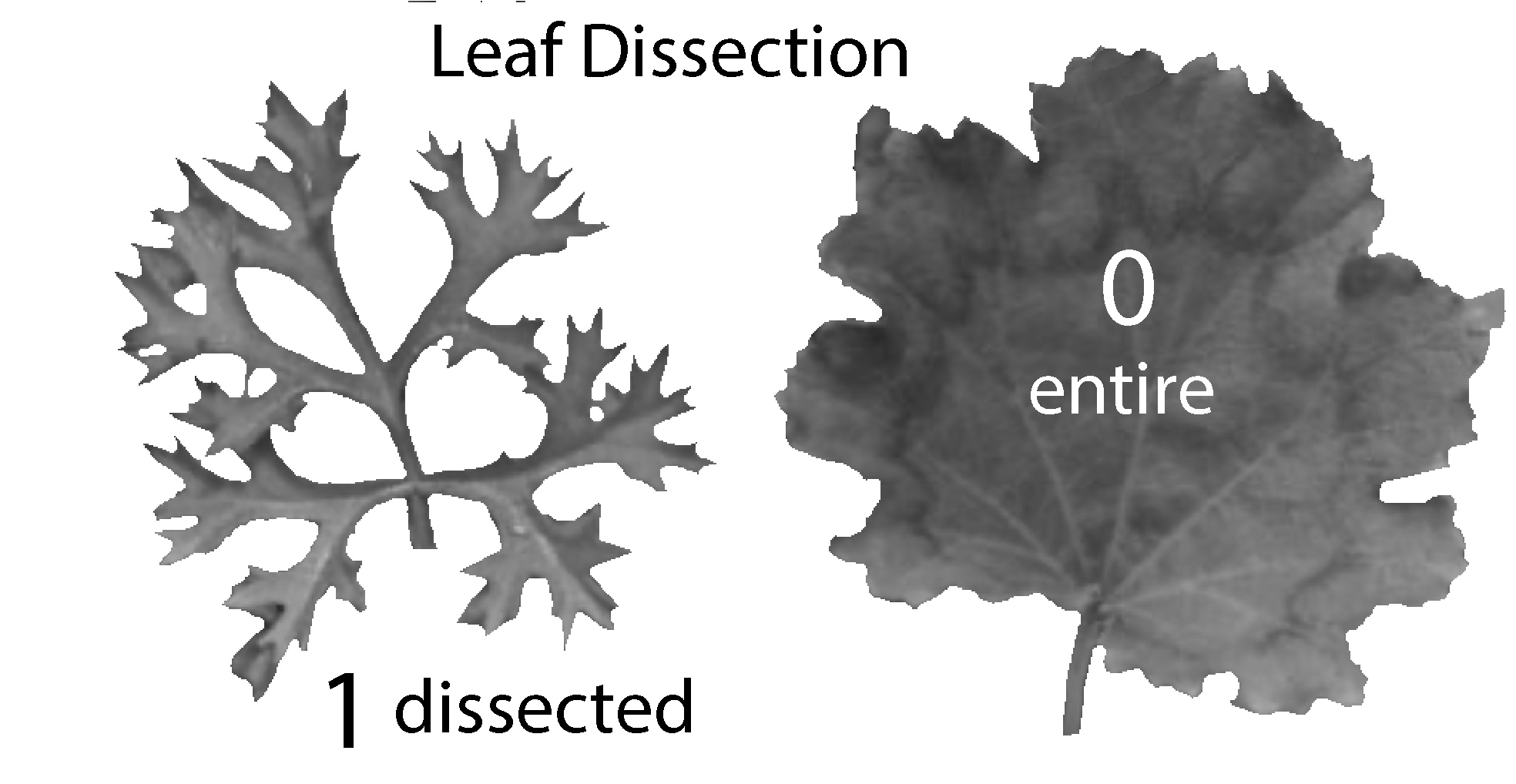
The leaf dissection trait comprises two states (I’ve merged some states in the original data matrix to produce just 2 states):
- 0 means leaves are entire (unlobed or shallowly lobed in the original study), and
- 1 means leaves are dissected (lobed, deeply lobed, or dissected in the original study).
Trait 2: Leaf venation
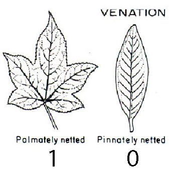
The leaf venation trait comprises two states:
- 0 means leaves are pinnately veined (one main vein runs down the long axis of the leaf blade), and
- 1 means leaves are palmately veined (several major veins meet at the base of the leaf).
First, we will use maximum likelihood to estimate the rates at which these two traits evolve under both an independent model (traits assumed to evolve independently) and a dependent model (the rates of change in one trait may differ depending on the state present in the other trait).
To test whether these two traits are correlated, we will carry out Bayesian MCMC analyses and estimate the marginal likelihood under two models. The model (independent or dependent) with the higher marginal likelihood will be the preferred model. You will recall that we discussed both of these models in lecture, and also discussed the stepping-stone method that BayesTraits uses to evaluate models. You may wish to pull up those lectures (as well as the BayesTraits manual) to help answer the questions that you will encounter momentarily.
Second, we will use reversible-jump MCMC to determine which of several thousand models is best. This method effectively uses marginal likelihoods to choose among models, but has the advantage that you need not specify which models you are interested in comparing beforehand.
Finally, I’ll show you how to estimate the marginal posterior probabilities of different ancestral state combinations using BayesTraits.
Maximum Likelihood: Independence model
![]() Type the following to start the BayesTraits program (assuming you are in the btlab folder):
Type the following to start the BayesTraits program (assuming you are in the btlab folder):
BayesTraitsV5 pelly.tre pelly.txt
You should see this selection appear:
Please select the model of evolution to use.
1)	MultiState
2)	Discrete: Independent
3)	Discrete: Dependant
4)	Continuous: Random Walk (Model A)
5)	Continuous: Directional (Model B)
6)	Continuous: Regression
7)	Independent Contrast
8)	Independent Contrast: Correlation
9)	Independent Contrast: Regression
10)	Discrete: Covarion
12)	Fat Tail
13)	Geo
![]() Press the 2 key and hit enter to select the Independent model. Now you should see these choices appear:
Press the 2 key and hit enter to select the Independent model. Now you should see these choices appear:
Please Select the analysis method to use.
1)	Maximum Likelihood.
2)	MCMC
![]() Press the 1 key and hit enter to select maximum likelihood. Now you should see some output showing the choices you explicitly (or implicitly) made:
Press the 1 key and hit enter to select maximum likelihood. Now you should see some output showing the choices you explicitly (or implicitly) made:
Options:
Model:                           Discrete: Independent
Tree File Name:                  pelly.tre
Data File Name:                  pelly.txt
Log File Name:                   pelly.txt.Log.txt
Save Initial Trees:              False
Save Trees:                      False
Summary:                         False
Seed:                            632248283
Analsis Type:                    Maximum Likelihood
ML Attempt Per Tree:             10
ML Max Evaluations:              20000
ML Tolerance:                    0.000001
ML Algorithm:                    BOBYQA
Rate Range:                      0.000000 - 100.000000
Precision:                       64 bits
Cores:                           1
No of Rates:                     4
Base frequency (PI's):           None
Pis used in ancestral state estimation:      Yes
Character Symbols:               00,01,10,11
Using a covarion model:          False
Normalise Q Matrix:              False
Restrictions:
    alpha1                       None
    beta1                        None
    alpha2                       None
    beta2                        None
Tree Information
     Trees:                      99
     Taxa:                       154
     Sites:                      1
     States:                     4
Checkpoint:                      False
Re Set Itterations:              False
Re Set Seed:                     False
![]() Now type
Now type run and hit enter to perform the analysis, which will consist of estimating the parameters of the independent model on each of the 99 trees contained in the pelly.tre file.
You will notice that BayesTraits created a new file: pelly.txt.Log.txt.
![]() Rename this file ml-independent.txt so that it will not be overwritten the next time you run BayesTraits:
Rename this file ml-independent.txt so that it will not be overwritten the next time you run BayesTraits:
mv pelly.txt.Log.txt ml-independent.txt
![]() Download the ml-independent.txt file to your laptop and use BBEdit (Mac) or Notepad++ (Windows) to view it. Scrolling past the first 36 lines, you should see the start of the parameter samples:
Download the ml-independent.txt file to your laptop and use BBEdit (Mac) or Notepad++ (Windows) to view it. Scrolling past the first 36 lines, you should see the start of the parameter samples:
Tree No	Lh	alpha1	beta1	alpha2	beta2	Root - P(0,0)	Root - P(0,1)	Root - P(1,0)	Root - P(1,1)
1	-157.362972	53.767527	34.523176	35.319157	20.707416	0.249998	0.250002	0.249998	0.250002
2	-158.179984	53.313539	34.182683	36.038859	20.997536	0.249999	0.250001	0.249999	0.250001
.
.
.
98	-156.647307	52.357626	36.749282	27.270771	13.086248	0.250244	0.249756	0.250244	0.249756
99	-156.532925	52.321467	36.641688	27.402067	13.200124	0.250234	0.249767	0.250233	0.249766
![]() Use your text editor to strip the first 36 lines, and open the file in Tracer.
Use your text editor to strip the first 36 lines, and open the file in Tracer.
Important note: while we are using Tracer to summarize, these results are from maximum likelihood analyses performed for each tree in the tree file. Because this is not a purely Bayesian analysis, you need not be overly concerned by the low ESS values reported by Tracer.
Answer these questions using the output you have generated. Here’s a key to the meaning of each column in the file:
| Column | Description |
|---|---|
| Tree No | Tree from pelly.tre |
| Lh | log-likelihood |
| alpha1 | leaf dissection: rate 0 (entire) -> 1 (dissected) |
| beta1 | leaf dissection: rate 1 (dissected) -> 0 (entire) |
| alpha2 | leaf venation: rate 0 (pinnate) -> 1 (palmate) |
| beta2 | leaf venation: rate 1 (palmate) -> 0 (pinnate) |
| Root - P(0,0) | prob. state 0,0 at root node |
| Root - P(0,1) | prob. state 0,1 at root node |
| Root - P(1,0) | prob. state 1,0 at root node |
| Root - P(1,1) | prob. state 1,1 at root node |
Which occurs at a faster rate: pinnate to palmate, or palmate to pinnate?
Maximum Likelihood: Dependence model
Run BayesTraits again, this time typing 3 on the first screen to choose the dependence model (note that “Dependant” should be “Dependent” in the menu) and again typing 1 on the second screen to select maximum likelihood. You should see this output showing the options selected:
Options:
Model:                           Discrete: Dependent
Tree File Name:                  pelly.tre
Data File Name:                  pelly.txt
Log File Name:                   pelly.txt.Log.txt
Save Initial Trees:              False
Save Trees:                      False
Summary:                         False
Seed:                            2700749663
Analsis Type:                    Maximum Likelihood
ML Attempt Per Tree:             10
ML Max Evaluations:              20000
ML Tolerance:                    0.000001
ML Algorithm:                    BOBYQA
Rate Range:                      0.000000 - 100.000000
Precision:                       64 bits
Cores:                           1
No of Rates:                     8
Base frequency (PI's):           None
Pis used in ancestral state estimation:      Yes
Character Symbols:               00,01,10,11
Using a covarion model:          False
Normalise Q Matrix:              False
Restrictions:
    q12                          None
    q13                          None
    q21                          None
    q24                          None
    q31                          None
    q34                          None
    q42                          None
    q43                          None
Tree Information
     Trees:                      99
     Taxa:                       154
     Sites:                      1
     States:                     4
Checkpoint:                      False
Re Set Itterations:              False
Re Set Seed:                     False
![]() Run the analysis. Here is an example of the output produced (in the file pelly.txt.Log.txt) after you type
Run the analysis. Here is an example of the output produced (in the file pelly.txt.Log.txt) after you type run to start the analysis:
Tree No	Lh	q12	q13	q21	q24	q31	q34	q42	q43	Root - P(0,0)	Root - P(0,1)	Root - P(1,0)	Root - P(1,1)
1	-151.930254	66.451053	37.783888	0.000000	62.220033	23.997490	23.299393	46.110432	36.632979	0.24999	0.249981	0.250026	0.250000
2	-152.925691	67.152271	38.611193	0.000000	60.925185	24.514488	23.937433	45.313366	37.199310	0.24999	0.249983	0.250023	0.250001
.
.
.
98	-150.816306	36.534843	27.359325	0.000000	66.563262	19.823546	24.944519	63.940577	31.074092	0.250048	0.249750	0.250304	0.249898
99	-150.712705	37.316351	27.260833	0.000000	64.364694	20.107653	25.004246	60.945163	31.658536	0.250030	0.249779	0.250272	0.249919
![]() Before doing anything else, rename the file pelly.txt.Log.txt to ml-dependent.txt so that it will not be overwritten the next time you run BayesTraits.
Before doing anything else, rename the file pelly.txt.Log.txt to ml-dependent.txt so that it will not be overwritten the next time you run BayesTraits.
mv pelly.txt.Log.txt ml-dependent.txt
Here’s a key to the rates:
| Rate | Context | Transition |
|---|---|---|
| q12 | dissection: 0 (entire) | venation: 0 (pinnate) -> 1 (palmate) |
| q13 | venation: 0 (pinnate) | dissection: 0 (entire) -> 1 (dissected) |
| q21 | dissection: 0 (entire) | venation: 1 (palmate) -> 0 (pinnate) |
| q24 | venation: 1 (palmate) | dissection: 0 (entire) -> 1 (dissected) |
| q31 | venation: 0 (pinnate) | dissection: 1 (dissected) -> 0 (entire) |
| q34 | dissection: 1 (dissected) | venation: 0 (pinnate) -> 1 (palmate) |
| q42 | venation 1 (palmate) | dissection: 1 (dissected) -> 0 (entire) |
| q43 | dissection: 1 (dissected) | venation: 1 (palmate) -> 0 (pinnate) |
Bayesian MCMC: Dependence model
![]() Run BayesTraits again, typing 3 on the first screen to choose the dependence model and this time typing 2 on the second screen to select MCMC. You should see this output showing the options selected:
Run BayesTraits again, typing 3 on the first screen to choose the dependence model and this time typing 2 on the second screen to select MCMC. You should see this output showing the options selected:
Options:
Model:                           Discrete: Dependent
Tree File Name:                  pelly.tre
Data File Name:                  pelly.txt
Log File Name:                   pelly.txt.Log.txt
Save Initial Trees:              False
Save Trees:                      False
Summary:                         False
Seed:                            2313422
Precision:                       64 bits
Cores:                           1
Analysis Type:                   MCMC
Sample Period:                   1000
Iterations:                      1010000
Burn in:                         10000
MCMC ML Start:                   False
Schedule File:                   pelly.txt.Schedule.txt
Rate Dev:                        AutoTune
No of Rates:                     8
Base frequency (PI's):           None
Pis used in ancestral state estimation:      Yes
Character Symbols:               00,01,10,11
Using a covarion model:          False
Normalise Q Matrix:              False
Restrictions:
    q12                          None
    q13                          None
    q21                          None
    q24                          None
    q31                          None
    q34                          None
    q42                          None
    q43                          None
Prior Information:
    Prior Categories:            100
    Priors
        q12 - uniform 0.00 100.00
        q13 - uniform 0.00 100.00
        q21 - uniform 0.00 100.00
        q24 - uniform 0.00 100.00
        q31 - uniform 0.00 100.00
        q34 - uniform 0.00 100.00
        q42 - uniform 0.00 100.00
        q43 - uniform 0.00 100.00
Tree Information
     Trees:                      99
     Taxa:                       154
     Sites:                      1
     States:                     4
Checkpoint:                      False
Re Set Itterations:              False
Re Set Seed:                     False
![]() Before typing run type the following command, which tells BayesTraits to change all priors from the default Uniform(0,100) to an Exponential distribution with mean 29:
Before typing run type the following command, which tells BayesTraits to change all priors from the default Uniform(0,100) to an Exponential distribution with mean 29:
pa exp 29
![]() Also type the following to ask BayesTraits to perform a stepping-stone analysis:
Also type the following to ask BayesTraits to perform a stepping-stone analysis:
stones 100 10000
![]() Now type
Now type run to start the analysis.
This will estimate 100 ratios to brook the gap between posterior and prior, using a sample size of 10000 for each “stone”.
Here is an example of the output stored in the file pelly.txt.Log.txt after you type run to start the analysis:
Iteration	Lh	Tree No	q12	q13	q21	q24	q31	q34	q42	q43	Root - P(0,0)	Root - P(0,1)	Root - P(1,0)	Root - P(1,1)
11000	-155.195365	78	14.423234	34.800270	8.845985	45.927148	12.622435	50.476188	52.844895	32.149168	0.250068	0.249969	0.249994	0.249968
12000	-154.161705	82	64.601017	12.382781	9.259134	51.796365	12.002095	23.744903	30.316089	21.865930	0.249936	0.249957	0.250095	0.250012 .
.
.
1009000	-154.343996	30	33.555198	50.086092	11.294490	38.518607	24.461032	47.295157	43.477964	21.726938	0.250057	0.249939	0.250045	0.249959
1010000	-154.195259	87	29.584898	35.410909	2.003582	61.981073	16.976124	14.895266	49.111354	14.419644	0.251115	0.247854	0.252551	0.248480
![]() Before doing anything else, rename the file pelly.txt.Log.txt to mcmc-dependent.txt, and pelly.txt.Stones.txt to mcmc-dependent.Stones.txt so that they will not be overwritten the next time you run BayesTraits.
Before doing anything else, rename the file pelly.txt.Log.txt to mcmc-dependent.txt, and pelly.txt.Stones.txt to mcmc-dependent.Stones.txt so that they will not be overwritten the next time you run BayesTraits.
mv pelly.txt.Log.txt mcmc-dependent.txt
mv pelly.txt.Stones.txt mcmc-dependent.Stones.txt
The Tree No column shows which of the 99 trees in the supplied pelly.tre treefile was chosen at random to be used for that particular sample point. BayesTraits appears to be sampling trees from the posterior distribution here; it cannot actually sample trees from the posterior because we have given it only data for two morphological characters, which would not provide nearly enough information to estimate the phylogeny for 154 taxa. It is as if we had given BayesTraits sequence data as well as our 2 morphological characters and it was using only the sequence data to estimate the posterior distribution of trees and edge lengths and only the morphological data to estimate rates for the morphological characters.
Answer these questions using the output you have generated:
Bayesian MCMC: Independence model
![]() Run BayesTraits again, this time specifying the Independent model, and again using MCMC,
Run BayesTraits again, this time specifying the Independent model, and again using MCMC, pa exp 29, and stones 100 10000.
![]() Rename the output file from pelly.txt.log.txt to mcmc-independent.txt. Also rename pelly.txt.Stones.txt to mcmc-independent.Stones.txt:
Rename the output file from pelly.txt.log.txt to mcmc-independent.txt. Also rename pelly.txt.Stones.txt to mcmc-independent.Stones.txt:
mv pelly.txt.Log.txt mcmc-independent.txt
mv pelly.txt.Stones.txt mcmc-independent.Stones.txt
Bayesian Reversible-jump MCMC
![]() Run BayesTraits again, specifying Dependent model, MCMC and, this time, specify the reversible-jump approach using the command
Run BayesTraits again, specifying Dependent model, MCMC and, this time, specify the reversible-jump approach using the command
rj exp 29
The previous command also sets the prior.
![]() Type
Type run to start, then when it finishes rename the output file rjmcmc-dependent.txt:
mv pelly.txt.Log.txt rjmcmc-dependent.txt
The reversible-jump approach carries out an MCMC analysis in which the number of model parameters (the dimension of the model) potentially changes from one iteration to the next. The full model allows each of the 8 rate parameters to be estimated separately, while other models restrict the values of some rate parameters to equal the values of other rate parameters. The output contains a column titled Model string that summarizes the model in a string of 8 symbols corresponding to the 8 rate parameters q12, q13, q21, q24, q31, q34, q42, and q43. For example, the model string “‘1 0 Z 0 1 1 0 2” sets q21 to zero (Z), q13=q24=q42 (parameter group 0), q12=q31=q34 (parameter group 1), and q43 has its own non-zero value distinct from parameter groups 0 and 1.
You could copy the “spreadsheet” part of the output file into Excel and sort by the model string column, but let’s instead use Python to summarize the output file.
![]() Download (e.g. using curl) the file btsummary.py and run it as follows:
Download (e.g. using curl) the file btsummary.py and run it as follows:
curl -O https://plewis.github.io/assets/scripts/btsummary.py
module load python
python3 btsummary.py
This should produce counts of model strings. (If it doesn’t, check to make sure your output file is named rjmcmc-dependent.txt because btsummary.py tries to open a file by that name.) Answer the following questions using the counts provided by btsummary.py:
Notice that many (but not all) model strings have Z for q21. One way to estimate the marginal posterior probability of the hypothesis that q21=0 is to sum the counts for all model strings that have Z in that third position corresponding to q21. While it is pretty easy to add these numbers in your head, let’s modify btsummary.py to do this for us (this might come in useful if you ever encounter results that are more complex).
![]() Open btsummary.py in nano and locate the line containing the regular expression search that pulls out all the model strings from the BayesTrait output file:
Open btsummary.py in nano and locate the line containing the regular expression search that pulls out all the model strings from the BayesTrait output file:
model_list = re.findall("'[Z0-9] [Z0-9] [Z0-9] [Z0-9] [Z0-9] [Z0-9] [Z0-9] [Z0-9]", stuff, re.M | re.S)
The re.findall function performs a regular expression search of the text stored in the variable stuff looking for strings that have a series of 8 space-separated characters, each of which is either the character Z or a digit between 0 and 9 (inclusive).
![]() Copy this line (in nano, you can do this with Ctrl-K (cut), Ctrl-U (uncut), Ctrl-U (uncut)), then comment out one copy by starting the line with the hash (#) character:
Copy this line (in nano, you can do this with Ctrl-K (cut), Ctrl-U (uncut), Ctrl-U (uncut)), then comment out one copy by starting the line with the hash (#) character:
#model_list = re.findall("'[Z0-9] [Z0-9] [Z0-9] [Z0-9] [Z0-9] [Z0-9] [Z0-9] [Z0-9]", stuff, re.M | re.S)
model_list = re.findall("'[Z0-9] [Z0-9] [Z0-9] [Z0-9] [Z0-9] [Z0-9] [Z0-9] [Z0-9]", stuff, re.M | re.S)
![]() Now modify the uncommented copy such that it counts only models with Z in the third position of the model string.
Now modify the uncommented copy such that it counts only models with Z in the third position of the model string.
model_list = re.findall("'[Z0-9] [Z0-9] Z [Z0-9] [Z0-9] [Z0-9] [Z0-9] [Z0-9]", stuff, re.M | re.S)
![]() Rerun btsummary.py, and now the total matches should equal the number of model strings sampled in which q21 = 0.
Rerun btsummary.py, and now the total matches should equal the number of model strings sampled in which q21 = 0.
Estimating ancestral states
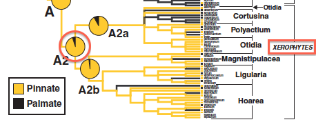
The Jones et al. 2009 study estimated ancestral states. In particular, they found that the most recent common ancestor (MRCA) of the xerophytic (dry-adapted) clade of pelargoniums almost certainly had pinnate venation (see red circle in figure on right). Let’s see what BayesTraits says.
![]() Start BayesTraits in the usual way, specifying 1 (Multistate) on the first screen and 2 (MCMC) on the second.
Start BayesTraits in the usual way, specifying 1 (Multistate) on the first screen and 2 (MCMC) on the second.
![]() After the options are output, type the following commands in, one line at a time, finishing with the run command:
After the options are output, type the following commands in, one line at a time, finishing with the run command:
pa exp 29
addtag xerotag alternans104 rapaceum130
addmrca xero xerotag
run
The addmrca command tells BayesTraits to add columns of numbers to the output that display the probabilities of each state for each character in the most recent common ancestor of the taxa listed in the addtag command (2 taxa are sufficient to define the MRCA, but more taxa may be included). The column headers for the last four columns of output should be (I’ve added the comments starting with <--)
xero - S(0) - P(0) <-- character 0 (dissection), probability of state 0 (entire)
xero - S(0) - P(1) <-- character 0 (dissection), probability of state 1 (dissected)
xero - S(1) - P(0) <-- character 1 (venation), probability of state 0 (pinnate)
xero - S(1) - P(1) <-- character 1 (venation), probability of state 1 (palmate)
![]() Download the output file (pelly.txt.Log.txt) and view it in Tracer.
Download the output file (pelly.txt.Log.txt) and view it in Tracer.
You can use Tracer to tell you the means of the four columns above. Note that you will need to remove the initial text from the file (but keep the column headers) before Tracer will recognize it.
That concludes the introduction to BayesTraits. A glance through the manual will convince you that there is much more to this program than we have time to cover in a single lab period, but you should know enough now to explore the rest on your own if you need these features.
What to turn in
Send your answers to the ![]() thinking questions to Analisa via Slack.
thinking questions to Analisa via Slack.